These are notes used for lecturing ECSE 507 during the Winter 2024 semester. Please note that these notes constantly evolve and beware of typos/errors. These notes are heavily influenced by Boyd and Vandenberghe’s excellent text Convex Optimization. I appreciate being informed about typos/errors in these notes.
N.B.: This page is formatted to be projected–see here for the unformatted version (i.e., without excessive whitespace).
Click each subject to unfold.
IntroductionGeneral Problem
Interested in solving and studying minimization problems subject to constraints:
where
are problem parameters;
is the objective function and usually interpreted as cost for choosing ;
is a constraint set often described “geometrically”.
Example 1. Design Problem Interpretation
Let
=scalar-valued design variables
(e.g., dimensions of manufactured object, yaw and pitch of jet).
= penalty for choosing design
(e.g., cost in material, energy, time, deviation from desired path).
= design specifications
(i.e., allowable/possible values for ).
E.g., specifies minimum and maximum design values.
Then the problem is to find optimal design values which minimize cost and satisfy the design specifications .
Example 2. Minimize function over ellipse
Let
.
Then the problem
is a familiar kind of purely geometric optimization problem.
It has two solutions: .
Many applied problems can look like this, but with an applied interpretation.
Problems With Structure
General optimization problems can be numerically inefficient to solve or analytically difficult, unless and have additional structure/properties.
Identifying nice structure/properties of problem problem may become analytically solvable or numerically efficient.
Examples of nice structure:
linearity defined in terms of linear equalities/inequalities;
e.g., , or succinctly written .
convexity or quasiconvexity
E.g., convex if is itself a convex set.
sparsity or other matrix structure
E.g., and given by
If sparse lots of cancellation improve computational efficiency
Linear Programming
Simplest case: is linear and defined in terms of linear constraints.
Notation: if , then
means for .
= transpose of the column vector . Linear program: given , , , solve
Thus and .
Positives of linear programming:
Conceptually simple: relies heavily on linear algebra
There are classical numerical methods which are often very efficient.
If is local minimizer of on , then it is automatically a global minimizer on .
Can sometimes approximate smooth problems linearly; however, usually can only give “local” results.
(E.g., for .)
Shortcomings of linear programming:
Many applied problems are not linear.
Many problems may not even be (suitably) approximated by linear programs.
E.g., the “barrier”
is better approximated by the a “logarithmic barrier” of the form than any linear function.
Convex OptimizationConvex optimization problem: and are convex.
This is the main focus of the course.
Positives of Convex Optimization:
Relatively conceptually simple.
Still often have efficient, albeit more sophisticated, numerical methods.
Many applied problems may be recast as or approximated by convex optimization problems.
If is local minimizer of on , then it is automatically a global minimizer on .
Shortcomings of Convex Optimization:
Problems may seriously fail to be analytically tractable or numerically efficient.
Exists nonlinear problems which cannot be approximated by convex problems.
Example (Least Squares)
A standard and ubiquitous kind of convex optimization problem is the least squares problem.
This problem takes the form:
where
is some norm
a matrix
a fixed vector
is the (convex) objective function
are convex.
N.B.: will come back to this problem.
Example: Distance from points to ellipse
If , is the identity matrix, and is an ellipsoid, then the solution is the point in the ellipsoid closest to the point .
The image below depicts this situation with
and .
Here, the optimal solution is .
Optimal Control
Let
be functions .
Assume evolves by
Here,
is the time derivative of .
are assumed to be given;
we think of as being the state of some system at time ;
we think of as an input we are allowed to choose to dictate the evolution of ; i.e., “controls” the system;
When , the system experiences “feedback.”
the goal: choose control law so that is as “desirable” as possible.
Example: Optimal Control ProblemsOptimal control problem: choose the “best” control which gives the “most” desirable .
Typically “best” and “desirable” are determined by size/cost of and ; e.g., one may wish to minimize
Therefore: problem is to solve (roughly speaking)
This will be another focus of the course and we will see some optimal control problems can be recast as convex optimization problems.
Rough Outline of Course
Part 1: Basics of Convexity and Convex Optimization Problems.
Part 2: Applications of Convex Optimization Problems.
Part 3: Algorithms for Solving Convex Optimization Problems.
Part 4: Topics in Optimal Control.
Convex GeometryConvex SetsConvex set: a subset satisfying:
for all and , there holds .
I.e., contains all line segments whose endpoints belong to .
Examples: some standard convex sets.
Closed or open polytopes in .
E.g., the interior of a tetrahedron.
Euclidean balls, ellipsoids.
Linear subspaces and affine spaces (e.g., lines, planes).
Given a norm on , the -ball
with center and radius is a convex set.
Recall: a norm satisfies
for all vectors ;
for all vectors and scalars ;
iff .
Affine SubsetsAffine subset: A subset satisfying:
For all and , there holds .
I.e., contains all lines which pass through two distinct points in .
N.B.: An affine subset is just a translated linear subspace:
“a linear space that’s forgotten its origin”. Example 1.
Let be the -plane in .
Then any translation or rotation of is an affine subset.
Example 2.
If , , then is affine.
( is just a translate of .)
Example 3.
Let
.
Then the solution set to is
,
which is just translated by 3 in the -direction:
ConesCone: A subset satisfying:
For all and , there holds .
I.e., contains all “positive” rays emanating from the origin and passing through any of its points. Proposition. is a convex cone iff for all and , there holds . Proof.
Step 1. ()
Suppose is a convex cone and let and be arbitrary.
Want to show: .
Step 2.
Being conic implies and belong to for all .
Step 3.
Being convex implies , as desired.
Step 4. ()
Suppose is such that for all and .
Want to show: is a convex cone.
Step 5. being conic follows from taking arbitrary and .
Step 6.
Convexity follows from taking with and .
Indeed: and for since .
Examples.
Hyperplanes with normal ,
halfspaces ,
nonnegative orthants are all convex cones.
(Here, if for .)
Given a norm on , the -norm cone is
,
which is a convex cone in .
See “positive semidefinite cone” below.
PolyhedraPolyhedron: Any subset of the form
given the vectors and scalars .
Thus, is a finite intersection of halfspaces and hyperplanes.
N.B.: Introducing equality constraints can be used to reduce dimension.
Example.
The polyhedron below is given by the indicated system of inequalities:
It is an easy exercise to rewrite the inequalities in the notation for suitable .
Positive SemidefinitenessSymmetric matrix:
a matrix satisfying ; i.e.,
Set of symmetric matrices:
Positive semidefinite matrix:
satisfying for all .
Equivalently, only has nonnegative eigenvalues.
If is positive semidefinite, then write .
If and , then write .
Set of symmetric positive semidefinite matrices:
(N.B.: is not the same as component-wise inequality, as was the case for vectors.)
Positive definite matrix:
satisfying if and only if .
Equivalently, only has positive eigenvalues.
If is positive definite, then write .
If and , then write .
Set of symmetric positive definite matrices:
Example 1
Let
.
Since has positive eigenvalues , it follows that .
To see explicitly, observe
with iff .
Example 2.
Let
.
Since has nonnegative eigenvalues , it follows that .
To see explicitly, observe
Evidently, for and so .
Example 3.
Let .
One can conclude by showing that has positive eigenvalues .
To see it directly, compute
But the discriminant (with respect to ) of this quadratic satisfies , from which we conclude the polynomial is positive unless and hence .
Example 4.
Let .
We can conclude , either compute its eigenvalues or observe that and whence cannot have only nonnegative eigenvalues.
Positive Semidefinite ConeProposition 1. is a -dimensional real vector space and is a convex cone in .Proof.Step 1.
is a vector space:
if and , then it is easy to see:
.
and so .
Step 2.
:
since implies , we have the identification
where the bolded entries in indicate the unique contributions to making .
Counting the number of bold entries shows has entries and hence .
Step 3.
is a convex cone:
For , and there holds
,
and so .
By the proposition in Convex Geometry.Cones, we conclude the desired result.
Proposition 2. iff
and .
Proof. Step 1.
Let
recalling that iff for all .
Step 2. (Case )
First compute
Observe that
for all iff .
Note (in case ): iff .
Can thus conclude (in case ):
for all iff .
Step 3. (Case )
Completing the square gives
But
for all
iff
and .
(To conclude , take .)
N.B.: strictly speaking, was not used anywhere; however, immediately implies , and also implies .
Step 4.
Putting Steps 2. and 3. together, we conclude: iff
and .
Image of
In light of Proposition 1 and Proposition 2, we can plot
.
The image below depicts the boundary of
.
Click to enlarge
Separating Hyperplanes
Let be two sets. Separating hyperplane: a hyperplane given by
for some and such that
is said to separate and .
Thus, cuts into two halfspaces with one containing all of and the other containing all of . Separating Hyperplane Theorem. If are two disjoint convex sets, then there exists and such that is a separating hyperplane which separates and .
Example 1.
Consider the convex sets
These three sets are indicated in the image below.
Note that separates the pairs and .
Moreover, the pair cannot be separated since and have significant overlap.
Example 2.
Consider the convex sets
These sets are indicated in the image below.
First note since neither contain their boundaries.
As such, they have a separating hyperplane which is given by .
N.B.: Replacing with their respective closures , the plane still separates .
Indeed, for and for .
Supporting Hyperplanes
Let be a fixed set and fix a boundary point
.
If the plane
separates and the singleton , then is called the supporting hyperplane of at .
Equivalently, lies entirely in a halfspace with boundary given by .
(Here: indicates the closure of and indicates its interior.)
Example.
Consider the convex sets
with boundary point .
Letting , we note .
Next, observing that, if , then and so
.
Thus separates and , showing that is a supporting hyperplane of at the boundary point ; see image below.
Hulls
Let be a fixed subset. Convex hull: the set
.
This is just the collection of all convex combinations of points in and is itself convex.
Example:
The images below depict a set of three points and its convex hull.
3 points in the plane
Convex hull of 3 points
Affine hull: the set
.
This is just the collection of all affine combinations of points in and is itself affine.
Example: The images below depict two points and their affine hull.
Two points in the plane
Affine hull of two points
Conic hull: The set
.
This is just the collection of all conic combinations of points in and is itself a cone.
Example: The images below depict two points , and their conic hull.
Two points in the plane
Conic hull of two points
Details
To see that the conic hull really is the shaded region, note that, by taking and , where and , the conic hull contains all points of the form .
Thus, it contains all line segments connecting any two points on the nonnegative rays and .
N.B.:
Conic hulls are convex cones.
Taking the “___ hull” of does indeed result in a “___” set.
The “___ hull” is a construction of the smallest “___” subset containing .
Generalized InequalitiesProper cone: a convex cone satisfying
is closed (i.e., contains its boundary)
has nonempty interior
.
Generalized inequality: given a proper cone , a partial ordering on defined by
.
N.B.: is a partial ordering and so is not well-defined for all .
Generalized strict inequality: given a proper cone , a partial ordering on defined by
.
Examples
(CO Example 2.14)
If , then is the standard componentwise vector inequality:
.
N.B.: is the standard inequality on .
(CO Example 2.15)
If , then
.
Let
.
Then is a proper cone.
In the image below:
is the cone with vertex .
The cone with vertex depicts those with .
The cone with vertex depicts those with .
N.B.: , and so , as indicated in the image.
Moreover, and are not comparable.
Convex Function TheoryConventions and Notations
Writing always means a partial function with domain possibly smaller than .
“Function” will mean “partial function.”
If , we may work with the extension given by
It is common to implicitly assume has been extended and to write for the partial function and its extension .
Given a set , its indicator function is
We write
Convex Functions
Let be a function with convex domain .
Convexity: for all there holds
(This inequality is often called Jensen’s inequality.)
Strict convexity: for all there holds
.
Example: failure of strict convexity
In the figure, the solid line indicates part of the graph of and the dashed line indicates part of the graph of a linear function.
This function fails to be everywhere strictly convex due to linear functions satisfying
.
Concavity and strict concavity: when is, respectively, convex and strictly convex.
Remarks.
It is instructive to compare convexity/concavity with linearity and view the former as weak versions of linearity.
It is common to extend the definition of convexity to extended functions, i.e., those of the form .
For example, the indicator function is convex in this sense.
To give insight, consider the image below, where the thick line is the “graph” of and the dashed line is the “secant line” connecting the points to for any .
Examples
All linear functions are convex and concave on their domains.
is convex on .
is convex on for .
is convex on for or and concave for .
is convex on
If is convex, then its indicator function is convex (in the extended value sense).
One Dimensional CharacterizationProposition.Let have convex domain and, given
and ,
define the function by
with
.
Then is convex iff is convex for all and such that is well-defined.
Proof.Step 1.
First note that is convex: it is the intersection of with the line passing through with direction .
Step 2. ()
Suppose is convex and let and be arbitrary.
Then, for and , there holds
proving that is convex.
Step 3. ()
Suppose now that each is convex.
Fix and let .
We want to show
.
Let and
,
noting that .
Since is convex, we conclude
This is enough to conclude is convex.
First Order CharacterizationProposition.If is differentiable with convex domain , then is convex iff
.
Proof (sketch).
We prove it in case ; the higher dimensional case follows by using that with convex domain is convex iff it is convex as a single variable function when restricted to lines intersecting .
Throughout, let and .
Step 1. ()
If is convex, then we obtain the following inequalities
Step 2. ()
Supposing
we set and add the two inequalities
to obtain
Remarks.
For fixed , the mapping
is affine whose graph is a hyperplane passing through the point .
Therefore, the inequality means this hyperplane is a tangent plane at of the graph of lying under the graph of .
In fact, this plane is a supporting hyperplane of the epigraph
at the point .
The affine mapping is just the first order Taylor approximation of at .
Thus, differential convex functions are such that their first order Taylor approximations serve as a global underestimators of .
Example.
In the image below:
solid line is the graph of ;
shaded region is the convex set given by ;
dashed line is the supporting hyperplane at given by the graph of .
gives a supporting hyperplane
Second Order CharacterizationProposition.If is twice-differentiable with convex, then is convex iff
.
Recall: if is twice-differentiable, then its Hessian is
Proof (sketch).Step 0.
The proof is a little more involved, so let us just give two intuitive justifications.
Justification 1.
The second order Taylor approximation gives
up to some small error.
But
implies
and so
(again, up to some small error).
The first order approximation from Convex Function Theory.First Order Characterization then implies convexity.
Justification 2.
Another intuitive justification is that means the graph of curves everywhere upward like a paraboloid, which evidently suggests convexity.
Remarks.
Recall: for , there holds
for all implies is strictly convex.
Converse is false since is strictly convex.
Level Sets
Fix a function and let -Level set: the set
.
The figure below depicts level sets of with
-Sublevel set:
the set
The figure below depicts the sublevel sets of with .
Each shade of gray indicates a new sublevel set and of course for .
-Superlevel set:
the set
.
The figure below depicts the superlevel sets of with .
Each shade of gray indicates a new superlevel set and of course for .
Proposition.If is convex, then the sublevel set is convex for all .
Equivalently, if is concave, then the superlevel set is convex for all .
Proof.
Want to show: implies for all .
If , then and so convexity of gives
and hence as desired.
Graphs
Fix a function .
Graph:
the set
.
Example: graph of is given below.
Epigraph:
the set
Example: epigraph of is given below.
Hypograph:
the set
Example: hypograph of is given below.
Proposition. is convex iff is convex.
Equivalently, is concave iff is convex.
Proof. (sketch)
We consider the case for simplicity. Step 1. ()
Suppose is convex and let be distinct points.
If both lie on a vertical line, then clearly for ; thus, suppose otherwise.
Let be the line passing through and let be the two intersection points of with the graph of .
(If at most one intersection point exists, then it is easy to see that the line connecting and is in .)
By convexity of , the line formed by for lies in , which is enough to conclude the line given by for lies in .
This shows is convex.
Step 2. ()
Suppose now is convex.
Let be two distinct points on the graph of .
Then .
But convexity of implies the line formed by for lies entirely in .
This is enough to conclude is convex.
Convex Calculus
The following list details some operations and actions that preserves convexity.
The main point: to conclude a function is convex, often one verifies may be built by other convex functions using, for example, the operations below.
N.B.: Conclusions only holds on common domains of the functions.
Conical combinations:
convex and
convex.
Weighted averages:
convex in , convex.
Affine change of variables:
convex, ,
convex.
Maximum:
convex
convex.
Supremum:
convex in for each
convex.
Justification.
For , there holds
Example.
Let
N.B.: for each , the mapping is affine and hence convex.
Thus
defines a convex function.
Infimum:
convex in
convex
finite for some
convex on
.
Fenchel conjugation
Let be given (not necessarily convex).
Fenchel conjugate: .
N.B.:
;
i.e., those for which is bounded above on as a function of .
Intuition.
Suppose is a differentiable convex function denoting the cost to produce items.
For a given unit price , the profit of selling units is
.
Thus is just the optimal profit for selling at price .
N.B.: convex implies is concave for each .
Thus, is maximal at satisfying , i.e., when .
Viz.: the where has slope .
The tangent line through is then given by .
Lastly, note that the -intercept of this line is ,
Remarks
Often is just called the conjugate function of .
Since is the supremum of a family of affine functions, is always convex, even if is not.
(Follows from Convex Function Theory.Convex Calculus.
If
is convex
is a closed subset of ,
then .
Example.
We will compute the conjugate function of
Thus, let
Case : is unbounded on since
as .
Thus
.
Case :
Compute
Thus maximizes and so
Case :
Compute
,
which evidently has least upper bound and so
Conclusion:
Since
is bounded on only for , it follows that
Putting everything together:
for ,
where we take .
Legendre Transform
Let be convex, differentiable and with .
Then, the Fenchel conjugate of is often called the Legendre transform of .
Proposition. If as above, and , then
.
Proof.Step 1.
Let
.
and note
maximizes iff
since is a sum of concave functions and hence concave.
Step 2.
Using Step 1. and
conclude
iff maximizes .
(In particular, maximizes .)
Step 3.
Letting satisfy
and using Steps 1. and 2., we conclude
,
as desired.
Example 1.
Let
,
and compute
.
Given , let
; i.e., .
Thus
,
which agrees with our calculation for in a previous example.
Example 2.
Fix and let
We will compute
.
Step 0.
Observe
is convex:
(Justification)
Consider case .
Let .
Thus .
Easy now to see .
implies is invertible since then .
Step 1.
Using
we conclude
Step 2.
Let .
By preceding proposition and Step 1., there holds
Other Notions of Convexity
There are two other important notions of convexity that we will return to if needed.
Let be given.
Quasiconvexity: and the sublevel sets
are convex for all .
Features:
Quasiconvex problems may sometimes be suitably approximated by convex problems.
Local minima need not be global minima
Log-convexity: on and is convex; equivalently
for all .
Generalized Convexity
Let be a proper cone and let .
-convexity: for all and , there holds
.
Strict -convexity: for all and , there holds
.
Examples
(CO Example 3.47)
Let .
Then is -convex iff: is convex and for all and , there holds
which holds iff
for each , i.e., iff is component-wisely convex.
(CO Example 3.48)
A function is -convex iff : is convex and for all and , there holds
.
N.B.:
this is a matrix inequality and -convexity is often called matrix convexity.
is matrix convex iff is convex for all .
The two functions
are matrix convex.
Basics of Optimization ProblemsGeneral Optimization Problems
By an optimization problem (OP) we mean the following:
We call
the objective function; the optimization variable or parameters; , , the inequality constraint functions; and , , the equality constraint functions.
The domain of (OP) is the intersection
.
Feasibility
Consider an (OP) as above. Feasible point: those satisfying
Feasible set: the subset consisting of the feasible points.
Feasible problem: A problem with nonempty feasible set, i.e., .
Infeasible problem: A problem with empty feasible set; i.e., there are no which satisfy the inequality and equality constraints.
Remark.
A feasible problem need not have a solution; e.g., has no minimizer nor minimum on .
An infeasible problem never has a solution–there are no parameters to even test.
Basic Example
Consider the problem
The objective function is
,
The inequality constraint functions are
.
The domain of the problem is
.
The feasible set:
Let
.
These three sets are depicted in the image below.
Note that the darkest region given by is the feasible set.
Can we solve the problem?
Noting
as approaches a point on the circle , and
such sequences exist in the feasible set,
we conclude the problem does not have a solution.
The Feasibility ProblemFeasibility problem: Given an (OP) with
solve
Viz.: the feasibility problem determines whether the constraints are consistent.
Example 1.
The problem
has a solution since the two inequality constraints describe two intersecting disks.
This is depicted below.
Example 2.
The problem
has no solution since the circle given by lies outside of the intersection of the two disks.
This is depicted below, where the red circle is given by .
Optimal Value and Solvability
Recall:
Optimal value:
The value
,
i.e., is the largest such that for all .
N.B.: .
Example:
Below depicts the graph of on .
Evidently, .
Solvable:
When the problem satisfies
there exists with ,
i.e., the minimum value is attainable.
Example:
Below depicts the graph of a quartic .
The problem of minimizing on is solvable with solution given by the minimal point .
N.B.: Point is a local minimum and hence does not give a solution.
Remarks.
iff the (OP) is solvable.
Indeed, is not well-defined unless the (OP) is solvable.
need not be finite:
if is unbounded below on the feasible set; and
if the OP is infeasible.
Standard Form
Optimization problems need not be placed in the form we defined them.
We therefore introduce the following definition.
(OP) in Standard form:
(This is how we defined (OP) before.)
Example: Rewriting in standard form.
We can recast more general optimization problems in standard form; e.g., consider
Indeed, taking
(noting )
for
for
we readily recast (OP2) into the standard form (OP).
Equivalent Problems
Suppose we are given two OP’s: (OP1) and (OP2).
We say (OP1) and (OP2) are equivalent if: solving (OP1) allows one to solve (OP2), and vice versa.
N.B.: Two problems being equivalent does not mean the problems are the same nor that they have the same solutions.
Example.
Consider the two problems:
Observing
minimizes on
iff
minimizes on ,
we readily see the two problems are equivalent.
Indeed, if we find the solution to the first problem, we readily obtain the solution to the second problem, and vice versa.
Change of Variables
Suppose is an injective function with .
Then, under the change of variable, we have
is equivalent to
N.B.: such a change of variables does not change the optimal value .
Moreover, injectivity may be dropped.
Justification.
Indeed,
if solves (OP1), then solves (OP2).
(More generally, such that solves (OP2).)
if solves (OP2), then solves (OP1).
Example
Consider the problem
.
In the image below, the shaded region is the feasible set and the curve is the graph of .
Consider the change of variables
.
The objective and constraints change as follows:
The new feasible region and objective function are plotted below.
Evidently, this change of variable changed a nonconvex (OP) into a convex one.
Eliminating Linear Constraints
Let , and a solution to .
Let be such that .
Then iff for some .
Consequently
is equivalent to
N.B.: this can reduce dimension of problem by many variables.
(Recall: .)
Justification.
Indeed,
if solves (OP1), then any with solves (OP2), and
if solves (OP2), then solves (OP1)
Example.
Consider the minimization problem
We may eliminate the variable by simply using .
But, to match with above: let
.
Thus
for some , and so
.
Therefore, the minimization problem becomes
which has the obvious solution with optimal value .
Thus, the original problem has solution
.
Slack Variables
Given with , then there is a variable such that ; such a variable is called a slack variable.
Using slack variables , the problem
is equivalent to the problem
Remarks.
All of the which may satisfy the constraints of (OP2) are the same as those which satisfy the constraints of (OP1); this justifies the equivalence.
Let be the feasible set of (OP1) and that of (OP2).
Then and ; i.e., the feasible sets are not the same object.
Example: in the images below, the disk depicts a feasible set and the paraboloid-type set depicts the feasible set with slack variable .
N.B.: the permissible coordinates are the same for both sets.
Main point:
Solving the system of equations
and considering only those solutions with may be easier than solving the system of inequalities
Example.
Consider
Introduce slack variable satisfying
.
Then (OP1) is equivalent to the problem
Thus, finding feasible is just a matter of solving a system of equations and choosing those with .
Moreover, one can solve the problem
and just choose solutions with to obtain solutions to (OP2), and hence (OP1).
Epigraph Form
Recall: .
The optimization problem
is equivalent to its epigraph form
Viz., minimizing subject to constraints is equivalent to finding the smallest such that for some feasible .
Proof by picture.
The dark curve and shaded region below indicate the epigraph of a function .
The red dot indicates the minimum point .
The black dots indicate points for different values of .
Evidently, the smallest for which is given by .
Fragmenting a ProblemProposition.Given and sets with let
Then
.
(Assuming for any real number .)
Viz., to minimize a function on a set , one may instead minimize over pieces of and then take the minimum optimal value of this procedure.
Example.
Consider the (OP)
where and where the feasible set is depicted below.
Consider breaking up into three regions as indicated below.
Now formulate the (OP)’s
for , and let be the optimal value for (OPi).
Using the preceding proposition, the optimal value of (OP) is given by
.
Conclusion: solving (OP), whose feasible set is not convex, may be achieved by solving three subproblems (OP1),(OP2),(OP3) whose feasible sets are convex.
Basics of Convex OptimizationConvex Optimization ProblemsAbstract convex optimization problem: A problem involving minimizing a convex objective function on a convex set. Convex optimization problem: a problem of the form
where
and are convex; and
and are fixed.
Some RemarksRemark 1.
As defined, a (COP) is an (OP) in standard form; naturally, there are nonstandard form (OP)’s equivalent to (COP)’s.
E.g., the abstract (COP)
is readily seen to be equivalent to the standard form (COP)
.
Remark 2.
We emphasize: the equality constraints are assumed to be affine constraints.
Moreover, the equality constraints
can be rewritten as
,
where
.
Remark 3.
The affine assumption on the equality constraints can be lifted at the possible expense of an intractable theory/numerical analysis.
E.g., if is quasilinear, then defines a convex set.
Remark 4.
Generally, convex does not imply the level set is convex; e.g., gives a sphere.
Remark 5.
The common domain
is convex since it is an intersection of convex sets.
Optimality for Convex Optimization Problems
Assume throughout that is the objective function for some given (COP) and that is the feasible set.
Proposition 1. If is a feasible local minimizer for a (COP), then it is the global minimizer for the (COP).Proof.
We will follow a proof by contradiction; i.e., we will show that assuming is not a global minimizer leads to a contradiction.
Step 1. being a feasible local minimizer means and that there is a such that
i.e., for all with a distance at most of .
Step 2.
Supposing is not a global minimizer, then there exists such that .
By choice of , there must also hold .
Step 3.
Set
noting that by Step 2. and so since is convex.
It follows that
Step 4.
Since is a convex combination of feasible points, since is convex and since , there holds
But, since minimizes on
and since
we also have
.
This is a contradiction and so must be a global minimizer.
Proposition 2.If is differentiable on , then is a minimizer iff for all there holds
.
Proof.Step 0.
N.B.: since is differentiable and convex on , then for each there holds
.
(C.f., Convex Function Theory.First Order Characterization.)
Step 1.()
Suppose is a minimizer and suppose for contradiction that
for some .
Set , noting that since is convex.
Using
,
we conclude is decreasing near in the direction and so for small .
Since , this contradicts being a minimizer.
Additional justification
Since defines a line passing through with direction , it follows that is the directional derivative in direction , i.e., .
Step 2.()
Supposing
for all and using the first order characterization at , namely,
we readily conclude
for all ; i.e., that is a minimizer for the problem.
CorollaryIn case is differentiable and (equivalently, there are no nontrivial constraints), is a minimizer iff
.
Proof.
By Proposition 2., we have that is a minimizer iff
for all .
Differentiability of requires is open and so, for small , there holds
.
But then
which is only possible for iff .
Some ExamplesExample 1.
Let
Consider the unconstrained problem:
.
Note that implies is convex.
C.f.,Convex Function Theory.Second Order Characterization.
By the preceding corollary, we have is a solution to (OP) iff
.
Thus solvability of (OP) rests on whether .
Three cases:
is unbounded below and hence (OP) is unsolvable;
is invertible and so is the unique solution to (OP);
and has an affine set of solutions.
Example 2.
Let
and consider the problem
.
Using a preceding proposition, satisfying is a minimizer iff
for all satisfying .
Two cases
is an inconsistent system the problem is infeasible.
is a consistent system; then
,
for some .
In case 2., we have
for all
and .
Since is a linear space, this is only possible iff
for all ,
i.e., iff
.
But and so this condition means there exists such that
.
This is just a Lagrange multiplier condition, as we will see later.
Linear ProgrammingLinear program: a (COP) of the form
,
where
The feasible set is a polyhedron (see below).
Recall ():
For the vector inequality
means
.
Different than: satisfying the matrix inequality, which means is positive semidefinite.
Determining the Feasible set:
Step 1. ()
Given , , then
is an affine subspace of or empty.
Step 2.
Given , then
is a half space in .
Step 3. ()
Given
Step 2. implies
is a finite intersection of half spaces.
Step 4.
Steps 1. and 3. imply the feasible to (LP) is the finite intersection of half spaces and an affine space, i.e., is a polyhedron.
(c.f. Convex Geometry.Polyhedra.)
Example.
Let
Consider the resulting (LP):
Explicitly, this (LP) is given by
The feasible set and the graph of the objective function over are indicated in the image below.
Remarks.
Given , have equivalent problem with objective .
Indeed,
WLOG: can assume to solve problem.
Since
one also calls the problem of maximizing over a polyhedron a (LP).
Example: Integer Linear Programming Relaxation.Integer Linear Program: an (OP) of the form
where
The constraint is suitable for parameters which take on discrete quantities.
N.B.: An (ILP) is not a convex problem, but may be approximated by one (see below).
The feasible set
Let
denote the feasible set of an (ILP).
Then is just the collection of integer vectors in the polyhedron
.
Example. Consider an (ILP) with constraints given by satisfying
The image below depicts the feasible set (the collection of dots) and polyhedron (shaded region).
Remarks.
Can of course also impose equality constraints :
If we impose , then the problem is called a boolean linear program:
Suitable for when coordinates of indicate when something is “off” or “on” or decision is “no” or “yes”.
Can also use instead.
Relaxation of (ILP)
The LP
is called a relaxation of the (ILP) and is a convex approximation.
Important points:
The “tightest” convex relaxation is given by
Generally speaking, finding the convex hull is not an efficient way of approaching (ILPs).
The relaxation (LP) of (ILP) is generally easier to solve, though exact algorithms exist for (ILP).
If
then .
(Indeed the relaxation has larger feasible set.)
If solves the (LP), then it solves the (ILP).
Relaxation of (BLP)
Explicitly, a (BLP) is of the form
The (LP)
is called a relaxation of the (BLP).
N.B.: the relaxation
generally provides a better approximation than the relaxation
.
Indeed, the former biases approximate solutions to be close to being binary.
Example.Problem Given workers and locations with ,
assign each worker to work at some location
assign at most one worker to a location
minimize cost of operation and transportation
Notational set up
Let
Construct objective function
We find
Thus the objective function is .
Construct constraints
The constraint that are binary is of course natural for the problem.
Since each worker is selected only once, we have
.
Lastly, observe since the th location not operating means it cannot host a worker; thus we have .
Formulate Problem
Putting everything together, the (BLP) formulation of the problem is
An (LP) relaxation (and hence convex approximation) of this (BLP) is
Quadratic ProgrammingQuadratic program: an (OP) of the form
where
If , then the problem is convex (see remarks).
Remarks.
As for (LP), the constraints
describe a polyhedron.
Given , then
WLOG: can assume to solve problem.
If
,
then
Thus implies is convex.
N.B.: The factor is just a convenient normalization.
The generalization
results in quadratically constrained quadratic programming (QCQP).
Imposing ensures the (QCQP) is convex.
(C.f., Convex Function Theory.Level Sets.)
The generalization
also results in a (QCQP), but this can break convexity.
E.g., The quadratic constraints
result in a (BLP) since these constraints enforce or , respectively.
There holds
The assumption (i.e., ) is not a serious restriction.
Indeed, first note that, since is a scalar, we have
.
Let
.
Thus,
where
.
Lastly, observe the symmetry of :
.
Thus every quadratic
has a “symmetric representation” of the form
with .
Example: Least SquaresLeast squares: an unconstrained (QP) of the form
where and .
Features:
WLOG: may assume columns of are linearly independent, and so
.
N.B.: a least norm solution to (LS) is generally given by
,
where is the pseudo-inverse (aka Moore-Penrose inverse) of .
Under the WLOG assumption, there holds
.
Recall (definition of )
For , the notation means the vector norm
.
Thus
is the distance between the two vectors .
Rough Justification of WLOG
Let
N.B.: a set of three 2-dimensional vectors is always linearly dependent and so
for some
Therefore, we may write
.
Computing
we see that minimizing
is equivalent to minimizing
Equivalence follows from the change of variables
.
Therefore, a (LS) problem with matrix of size is equivalent to a (LS) problem with matrix of size .
This argument holds in general: if has linearly dependent columns, can use change of variables to ensure linear independence.
Remarks.
If has solution , then solves the (LS) problem.
If has no solution, then any solving the (LS) problem gives a “best” estimate solution to , where “best” is chosen to mean in terms of the vector norm .
While minimizing is equivalent to minimizing , the exponent ensures is differentiable (at ).
(C.f.: is not differentiable at , but is.)
Solving the (LS)Step 1. (The problem is convex)
The objective function
is convex since
.
To see , observe:
and so , i.e., is symmetric;
for all there holds
,
i.e., .
Step 2. (The critical points)
We compute
Therefore, iff
.
This system of equations consists of what are called the normal equations.
Step 3. (The solution)
By corollary proved above: is a solution iff .
Moreover, having linearly independent columns ensures that is invertible:
linear independent columns iff .
.
Since is square, can conclude is invertible.
Lastly: since
iff
and since is invertible, we conclude that the solution to the (LS) is
.
Example: Distance Between Convex Sets
Let be convex subsets. Nearest Point Problem (NPP): Among , which pair minimizes the distance ?
The (NPP) may be expressed as a standard form (COP).
Indeed, supposing
with convex, then the (NPP) for is the (COP)
N.B.: the feasible set is
Viz.: iff .
When the are polyhedra, then the (NPP) is a (QP).
Indeed, supposing
then the (NPP) for is the (QP) given by
Can formulate as constrained least squares problem: defining
we readily see that the problem is equivalent to
Polyhedral Approximation.
Let be nonempty convex domains, not necessarily polyhedral.
Let be polyhedral domains such that
Then the (NPP) for the pairs and provide (QP) relaxations of the (NPP) for and, respectively, provide upper and lower bounds for the optimal values for the original (NPP).
Geometric ProgrammingMonomial function: given
,
a function of the form
Example.
.
Posynomial: given
,
a function of the form
Example.
Geometric Programming: An (OP) of the form
where
N.B.: this is an undercover (COP).
Remarks.
Let
Since any monomial is a posynomial, we have .
If
then
Thus is a group and a “conic representation” of .
As usual, we use the language “writing in standard form” to refer to writing an equivalent (OP) written in the form (GP) above.
General (OPs) clearly equivalent to a (GP) may be called a geometric program in nonstandard form.
For example, the geometric program
with
is readily rewritten as a standard form (GP):
Rewriting (GP) as a (COP)
General (GPs) are not convex (e.g., ).
However, any (GP) is easily recast as a (COP) via change of variable.
Step 1. (The change of variable)
We will write to mean the change of variable given by
Step 2. (Monomials convex function)
Let
Under the change of variable :
But
convex convex
and so is convex since affine functions are convex.
Step 3. (Posynomial convex function)
For , let
By Step 2., there holds
which is again a convex function.
Step 4. ((GP) (COP))
We explicitly write the (GP) as:
Let
Under the change of variable , this (GP) becomes the (COP)
Step 5. ((GP) in convex form)
At last, since exponentiation may result in unreasonably large numbers, it is customary to take logarithms, resulting in the geometric problem in convex form:
N.B.:
Concavity of is too weak to break the convexity of , and so the problem is still convex.
The constraints are equivalent since is monotonic and injective on .
Example.(Taken from Boyd-Kim-Vandenberghe-Hassibi: A tutorial on geometric programming) Problem Maximize the volume of a box with
a limit on total wall area;
a limit on total floor area; and
upper and lower bounds on the aspect ratios and .
Notational set up
Construct objective function
The volume of the box is
and so the objective function is
.
N.B.:
Construct contraints
N.B.:
Formulate Problem
Putting everything together, we realize the problem may be formulated as the following (GP):
To write the problem in standard form: note the following equivalence of constraints
Moreover, maximizing is equivalent to minimizing .
Therefore, the problem in standard form is given by
Semidefinite Programming
(Heavily influenced by Vandenberghe-Boyd Semidefinite Programming.) Linear matrix inequality (LMI): given
an inequality of the form
.
Recall: for , we write to mean is positive semidefinite, i.e., for all .
Semidefinite program (SDP): an (OP) of the form
where
N.B.: The LMI defines a feasible set which is convex and hence (SDPs) are convex problems.
Convexity of Feasible Set.
To see that (SDP) is a convex problem, first note: if
and
then
and so
.
Next, observe: for feasible and , the function
evaluated at the convex combination
is
Expanding, rearranging and using
gives:
Using , we conclude
.
Thus, feasible feasible for , i.e., the feasible set is convex.
Example 1. LPs are SDPs
Consider the (LP)
where
and
means componentwise inequality.
Given , define
Since satisfies iff has nonnegative eigenvalues, we have
.
(Indeed, the eigenvalues of are the components of .)
Therefore,
Letting
,
we have
.
Therefore, using
we have
Therefore, defining
we conclude
.
In conclusion, we have that the (LP)
is equivalent to the (SDP)
Example 2. Nonlinear OP as a SDP
Consider the nonlinear (COP)
where
We will recast (OP1) as a (SDP).
N.B.:
choice of domain (a halfspace) of objective and ensures convexity.
concave problem.
To begin, recall we may recast problem in epigraph form:
N.B.: this introduces the new optimization variable .
Goal: find a symmetric matrix-valued function
such that the constraints
may be recast as the LMI
Idea: we know
.
On the other hand:
.
Recall: if , then
Therefore, given , we have
.
Using that
we therefore introduce
to capture the problems constraints.
Indeed, evidently, iff
and .
Therefore,
.
This is enough to conclude (OP1) may be recast as an (SDP).
To make it clearer, introduce the notation
and matrices
Then
and so (OP1) is equivalent to the (SDP)
Lagrangian Duality
Throughout, let (OP) denote a given optimization problem of the form
Recall:
The Lagrange DualLagrangian: the function
given by
.
N.B.: for each fixed , the function
is affine.
Lagrange multipliers: the variables and .
The vectors
are called dual variables.
Lagrange dual function: the function
given by
.
Those satisfying
are called dual feasible.
N.B.: as an infimum of affine functions, is automatically concave.
Proposition. For
,
there holds
,
where is the optimal value for the given (OP).
Proof.
Let be feasible.
Then
Let and be arbitrary.
Then feasibility of implies
Consequently,
Therefore, for all feasible , for and for arbitrary , there holds
and so
.
(Indeed, is a lower bound of and is the greatest lower bound of .)
Lagrangian as underestimator. (See CO 5.1.4)
Define the indicator functions
Then
and the (OP) is equivalent to
N.B.: the terms in
act as penalties for breaking the desired constraints.
N.B.: if is feasible and , then
and hence
.
Viz., is an underestimater of the objective function
obtained by “softening” or “weakening” the penalty functions:
In particular, for each , the problem
has optimal value and provides an underestimation of the original (OP).
Example 1
Consider the least squares problem
for given
.
N.B.:
.
Therefore, the Lagrangian for (LS) is
and the Lagrange dual is
N.B.:
and so is convex.
Consequently,
iff
,
i.e., iff
In conclusion,
In particular,
for all .
Example 2
Consider the linear program
for given
.
N.B.:
equality constraints given by
.
iff
iff
.
Therefore, the Lagrangian for (LP) is
Want to compute
but
is an affine function with domain .
Therefore,
is bounded below iff satisfy
.
Therefore, the Lagrange dual is
In particular, for dual feasible , there holds
for all feasible .
Return of Conjugate Function
Recall: given , its conjugate function is the convex function
Interestingly: the conjugate function is related to the Lagrange dual.
Example.
Consider the the (OP)
for given
We may write
for suitable
The Lagrangian is
We may now compute the Lagrange dual in terms of the conjugate :
Since
,
we conclude
Example: A Volume Minimizing EllipsoidProblem. Given points , among all (closed) origin centered ellipsoids satisfying , find those with minimal volume.
Plan. We will formulate this problem as a convex optimization problem and determine the Lagrange dual function.
Positive semidefinite representation of ellipsoids.
Given , the set
is an ellipsoid.
Moreover, the volume of is proportional to .
(This follows change of variable formula.)
Justification
WLOG: for some whose entries are the positive eigenvalues of .
Then implies
which is the usual description of a closed ellipsoid with center .
E.g., gives the ball of radius .
Problem reformulation. Find those satisfying which minimize .
In fact, is convex, and so we may reformulate the problem as the following (COP):
Recall
for ;
there is a natural way of identifying matrix with vector ;
Under this identification, we have
.
Let , noting .
Then 1. gives
Therefore 2. and 3. allow us to realize the quadratic inequality
as the linear inequality
.
These observations allow us to appeal to the Lagrange dual formalism.
It can be shown
From preceding section, we can conclude the Lagrange dual function of is
Since provides a lower bound of the optimal value, we conclude: if is the optimal volume, then, up to known constant , there holds
,
which is a very explicit lower bound depending only on the Lagrange multiplier and the problem data.
Let
.
Therefore, the problem is equivalent to
Introducing the Lagrange multiplier , observe
.
Under our chosen identification , we identify
and so
We lastly record the conjugate function of :
.
By previous section, the Lagrange dual is given by
.
Since provides a lower bound of the optimal value, we conclude: if is the optimal volume, then, up to known constant , there holds
,
which is a very explicit lower bound depending only on the Lagrange multiplier and the problem data.
The Dual Problem
Let
Recall
Main point:
,
suggests considering maximization problem with objective .
Gives best underestimate available by Lagrange dual function.
Lagrange dual problem: the problem
Remarks
The original problem is called the primal problem.
Viz.., the dual problem is dual to the primal problem.
feasible to dual problem .
Viz., is dual feasible.
As stated, the only constraint is ; however, domain of usually has implicit constraints.
Generally: has “dimension” less than or equal to .
Recall: is infimum of family of concave functions.
Thus, is concave and is convex.
So,
maximizing concave minimizing convex .
Therefore, since is convex constraint:
Dual problems are always convex, even if primal is not.
Solutions to dual are called dual optimal.
Remark on Duality for Equivalent ProblemsQuestion: if two primal problems are equivalent, how are their respective duals related?
Spoiler: The respective dual problems may be quite different; this is demonstrated by example.
Example. Consider the unconstrained problem
This problem is equivalent to the constrained problem
Having no constraints, the Lagrangian for (OP1) is
and so the Lagrange dual function is simply
Therefore, the dual problem of (OP1) trivializes to minimizing a constant.
Having only the equality constraints , the Lagrangian for (OP2) is
.
Observe that is unbounded below if .
Moreover, if , then
Thus,
Therefore, the dual problem to (OP2) is
Conclusion: the dual of (OP2) is conceivable useful, whereas the dual of (OP1) is useless, even though (OP1) and (OP2) are equivalent.
Example: Duality of standard form and inequality form LP
Recall: a standard form LP is of the form
.
An inequality form LP is of the form
.
We will show the dual of (LP1) is (equivalent to a problem) of the form (LP2), and vice versa.
The dual (LP1)
We consider first:
.
For (LP1), the Lagrangian is
and Langrange dual function is
.
(Recall: domain is determined by where is bounded below.)
Therefore, the dual problem of (LP1) is
which is evidently equivalent to
N.B.: the domain of had the implicit constraint .
Observe the equivalency of constraints:
Therefore
The last problem is of the form (LP2).
Viz., the dual of a standard form LP is (equivalent to) an inequality form LP.
The dual of (LP2)
We now consider
.
For (LP2), the Lagrangian is
.
N.B.: an affine function is bounded below iff .
Therefore, the Lagrange dual function is
.
Therefore, the dual problem of (LP2) is
which is evidently equivalent to
Again, the domain of had an implicit constraint, namely, .
Observe the equivalency of constraints:
Therefore, the dual problem is equivalent to
which is a problem of the form (LP1).
Viz., the dual of an inequality form LP is a standard form LP.
Weak and Strong Duality
Let
Weak duality: the property .
N.B.: Optimization problems of the form (OP) always satisfy weak duality. Strong duality: the property .
N.B.: Having strong duality does not mean the primal and the dual are actually solvable. Constraint qualifications: conditions for a given type of problem which ensure strong duality.
E.g., “A (QCQP) with single quadratic constraint has strong duality if _______.” Optimal duality gap: the difference .
Remarks
Observe
Therefore
is possible.
Primal and dual may be simultaneously infeasible, i.e.,
may occur.
Convex optimization problems often have strong duality, but not always.
Slater’s Condition
Consider the (COP)
with domain .
Let denote the relative interior of .
Intuitively: means is not on the “boundary” of
Recall: generally has smaller dimension than number of variables.
Slater’s condition: there exists such that
and .
Strict feasibility: when a feasible satisfies Slater’s condition.
Example
Consider the inequality constraints
and suppose has
.
Then is feasible but not strictly feasible.
Moreover, any point in the interior of the smallest disk satisfies Slater’s condition.
Slater’s Theorem. If (COP) satisfies Slater’s condition, then it is strongly dual and the dual problem is solvable
Remarks.
Slater’s condition is a constraint qualification for convex optimization problems.
In principle, an (OP) may be strongly dual without the dual being solvable.
Thus, Slater’s theorem has the strength of implying there is a dual feasible with .
Theorem. If Slater’s condition holds for all non-affine inequality constraints, then conclusion of Slater’s theorem hold.
Remarks.
Thus, if are affine and are not, then it is enough if there holds the weakened Slater condition: there exists a such that
.
Therefore, Slater’s condition is really a qualification constraint for non-affine inequality constraints.
Remark on Slater’s Condition
Consider the convex optimization problem
Let be the domain.
Since is convex, it lies in its affine hull .
Given ,
be the Euclidean ball of radius and center . Relative interior: the set
Example. In the image below:
is the ellipse lying in the -plane.
The affine hull is the -plane.
The ball depicts a ball centered at a point in and with small enough radius so that still lies in .
The relative interior is the shaded region of the ellipse excluding the curve bounding the domain.
Question How can Slater’s condition fail?
I.e., what if there exist no such that
Consider the (COP)
where are convex.
Suppose
describes a cube:
,
the solution set
is a plane intersecting the top face of the cube.
The images below depict the cube, the plane and their intersection (a square).
N.B.: the domain is the area below and including the plane.
Then the domain is and (COP) fails Slater’s condition:
if , then must fail.
Fix: Can project problem onto a lower dimensional face of .
Indeed, since
,
(COP) is equivalent to the problem
where .
Taking , we see (COP1) satisfies Slater’s condition.
Comparing Duals and KKT Conditions.
Let and be the Lagrangian for (COP) and (COP1) respectively.
Then
The respective KKT conditions are
Remarks.
While (COP) does not satisfy Slater’s conditions, its projection (COP1) does.
might not even be differentiable, in which the KKT conditions for (COP) would be ill-posed.
Identifying the correct face to project problem to relatively simpler KKT conditions.
(Not true in general.)
Geometric description of Slater’s condition failing:
Consider a general (COP) with convex domain .
Suppose the relative boundary of contains a convex set (e.g., a polygonal face or is conic)
If or , then the problem fails Slater’s condition.
Indeed, any feasible point must satisfy and lie on the relative boundary (and hence not in the relative interior).
N.B.: a problem even “almost” failing Slater’s condition can cause numerical issues.
E.g., a 3-dimensional problem with nearly 2-dimensional domain.
ExamplesExample 1.
Consider the least squares problem
Recall: the Lagrangian is
and Lagrange dual function is
.
Therefore, the dual problem is
N.B.: (LP) has no inequality constraints and .
Thus, Slater’s condition is simply:
there exists such that , i.e., .
We will analyze this closer.
Case 1 ():
Here, Slater’s condition is satisfied since implies there exists with .
Therefore, primal is feasible and hence .
Slater’s theorem implies
.
In particular, the dual objective
is bounded above.
Case 2 ():
Here, the primal is infeasible and so .
Note exists such that and .
(Recall: .)
But then
,
which is unbounded above as a function of , and so .
In conclusion: for (LS), there holds , even when .
Therefore, (LS) is strongly dual whether feasible or infeasible.
Example 2.
Consider the standard form (LP)
We have already shown that its dual problem is
Since the inequality constraints of (LP) are affine, namely,
weakened version of Slater’s condition implies problem is strongly dual when feasible.
Interestingly: (LP) may fail to be strongly dual when infeasible, i.e., there may hold and .
Example 3.
Consider the QCQP
where
We now determine the dual problem.
The Lagrangian of (QCQP) is
Defining
we have
.
We now compute the Lagrange dual function for .
To begin, observe: if , then
due to positive semidefiniteness of .
So: is invertible and
.
is convex in .
Therefore, is determined by critical points of .
Compute
Thus, is a minimizer of iff
.
Therefore,
Therefore, the primal problem
has dual problem
Slater’s theorem implies that these two problems are strongly dual if there exists a strictly feasible satisfying
for all .
Qualitative Uses of Lagrange Duality
Recall: a problem has
These are qualitative properties; e.g., strong duality alone does not provide means to find primal optimal satisfying ;
However, strong and weak duality provide three useful “qualitative” uses:
Certification: a dual feasible provides a certification that is a suboptimal value: .
Strong duality can (theoretically) certify up to any desirable precision.
Duality gap: for primal feasible and dual feasible , the value
.
N.B.: if feasible, then
i.e.,
and the duality gap gives length of interval.
In particular: if duality gap at a feasible pair , then
give
,
i.e., such certifies that is optimal, and vice versa.
Stopping Criterion. Observing
and setting
we see
Viz.,
.
N.B.: this is showing is -suboptimal without even knowing the primal optimal .
As application: suppose we wish to find optimal but can settle for feasible with at worst -suboptimal:
.
Suppose we use algorithm producing feasible in search of optimal .
Letting
denote the resulting duality gaps, we may use the following stopping criterion:
.
Therefore, with gives feasible within allowed error: .
N.B.:
Re-emphasize: this stopping criterion does not require knowing the primal optimal in advance.
strong duality can be arbitrarily small.
Complementary slackness. Assume problem has strong duality, i.e., .
If is primal optimal and is dual optimal, then
.
For example:
where is the vector of inequality constraint functions.
This relationship between the two vectors is called complementary slackness.
N.B.:
Since and , we have
While a qualitative property, complementary slackness can sometimes be used to solve the primal.
Having is permissible.
Justification: for primal optimal and dual optimal, we find
Since
,
and since , we conclude
and so
Since and , the sum
is a sum of nonpositive things and so
implies
which is the desired complementary slackness.
Karush-Kuhn-Tucker (KKT) Conditions
Assume are differentiable and have open domains.
In previous section, we saw: if are optimal with zero optimality gap, then
Question: What does this say about relationship between , and (under strong duality)?
Above is equivalent to:
.
or
.
Viz., if
problem is strongly dual,
is primal optimal, and
is dual optimal,
then minimizes the Lagrangian with dual optimal Lagrange multipliers.
But, if
minimizes and
are differentiable,
then is differentiable and is a critical point:
Beware: we do not know a priori if or are zero.
Karush-Kuhn-Tucker (KKT) Optimality Conditions:
Recap:
these are necessary conditions for any strongly dual optimization problem admitting primal optimal and dual optimal
the first and second conditions just indicate is primal feasible;
the third condition is the complementary slackness derived in previous section;
the fourth condition is standard nonnegativity of Lagrange multiplier
the last condition follows from minimizing .
KKT and ConvexityTheorem.
If the primal problem is differentiable and convex, then the KKT conditions are sufficient for primal and dual optimality and strong duality.
Viz., for differentiable convex problems, if and satisfy the KKT conditions, then they automatically primal and dual optimal, respectively.
Proof.Step 1. Suppose and satisfy the KKT conditions:
First two conditions is primal feasible.
Step 2. Observe
are convex.
Thus
.
as a function of is a sum of convex functions and hence convex.
Therefore is a minimizer.
This also implies is dual feasible since
.
Step 3. By Step 2., feasibility of and the complementary slackness
there holds
Therefore, the duality gap vanishes and hence is primal optimal and is dual optimal.
Indeed, recall:
and so implies
Corollary.
If the primal problem is differentiable, convex and satisfies Slater’s condition, then the KKT conditions are necessary and sufficient for primal and dual optimality and strong duality.
Viz.: in this situation, finding all solutions to KKT conditions provides all solutions to the given problem.
Remark. In convex optimization, many algorithms are conceived as methods for solving KKT conditions.
Moreover, some KKT conditions for some problems may be solved analytically.
Example 1(CO Example 5.1)
Consider the quadratic program
with .
Goal: Derive the KKT conditions for (QP) and solve (QP).
Step 0. Observe that (QP) is a differentiable convex problem which trivially satisfies Slater’s conditions and so the KKT conditions may be used to solve it.
Step 1. Find the Lagrangian and its gradient:
(QP) only has the equality constraint and so the Lagrangian is
.
Differentiating with respect to gives
Step 2. Construct the KKT conditions:
Since (QP) has no inequality constraints, the KKT conditions take the form
Viz., the KKT conditions for (QP) are
Rewriting the KKT conditions as
the KKT conditions are evidently equivalent to the matrix equation
Conclusion: Solving the quadratic program
is equivalent to solving the linear equation
Example 2(CO Example 5.2)
Consider the convex optimization problem
where and is the vector of 1’s.
Goal: Derive the KKT conditions for (WF) and solve (WF).
Step 0. Observe
the domain of (WF) contains the nonnegative orthant .
(WF) is a differentiable convex problem.
The condition is equivalent to .
(WF) satisfies Slater’s condition since there exist with and so (WF) satisfies strong duality.
Therefore, we may use KKT conditions to solve (WF).
Step 1. Find the Lagrangian and its gradient:
Given the constraints
the Lagrangian is
with Lagrange multipliers
.
Differentiating with respect to gives
Thus, is a critical point of if it satisfies the system of equations
Step 2. Construct the KKT conditions:
Since (WF) has inequality and equality constraints, the KKT conditions take the form
Thus, the KKT conditions for (WF) are
Observe:
is equivalent to
(In particular, is acting as a slack variable.)
Therefore, we wish to solve:
We will solve for in terms of by considering two cases.
Case 1: .
Observe
is only possible for if .
Then the complementary slackness
enforces .
Case 2:
If , then
and so the complementary slackness
furnishes the contradiction .
Thus .
Putting the two cases together:
Next, using , we get
This is enough to solve for and hence .
Further details: Consider the function
with .
Observe
and so on.
Moreover, is continuous.
Thus is an increasing continuous piecewise linear function.
Then may be solved by finding when the graph of crosses the horizontal line .
Perturbation
Given the OP:
a natural question is:
How do and behave under perturbations of constraints?
More precisely: given , , consider the perturbed problem
Observe
results in ;
results in relaxing ;
results in tightening ;
results in “translating” solution set of .
Example 1.
The image below depicts various perturbations in inequality constraints (the shaded regions) and equality constraints (the dashed contours).
N.B.: perturbing the equality constraint results in using different contours.
Example 2.
The three images below depict the constraint
with , respectively.
The three images below depict the constraint
with , respectively.
The optimality function
For and , let denote the primal optimal value for .
Can therefore introduce the function
which assigns perturbation the primal optimal value .
N.B.:
primal optimal value of unperturbed problem;
If , then the perturbation makes the problem infeasible.
If , then the perturbation makes the problem unbounded.
If (OP) is convex, then is convex in .
Example
Consider the problem
Given and the constraint, problem is:
minimize on .
Evidently, .
Consider now the perturbation
Viz.,
minimize on .
Given , perturbed problem is feasible only for .
Can thus conclude
The graph of is plotted below; observe the behavior of as the constraint is relaxed.
SensitivityTheorem. If the primal has strong duality and the dual optimal is achieved by dual feasible , then
for any and .
Proof.
Fix the perturbation vector and let be feasible for the resulting perturbed problem:
Observe:
Using this and strong duality gives
Rearranging gives
for all feasible for the perturbed problem.
Since LHS independent of , there holds
Remark. Using this theorem, the sizes and signs of may determine the sensitivity of the primal optimal value subjected to perturbation.
Example
Suppose Theorem inequality takes the form
.
We make four observations.
The larger is, the easier tightening results in increasing .
Consider :
The smaller is, the more flexibility we have to relax without decreasing too much.
Consider :
When : the larger is, the easier changing increases .
Consider :
When : the smaller is, the more flexibility we have to change without decreasing too much.
Consider :
Example
This example reviews KKT conditions, Slater’s condition, perturbation and sensitivity.
Consider the LP
where is fixed.
The Lagrangian and its gradient
Since the constraints are
the Lagrangian takes the form
Differentiating with respect to gives
KKT Conditions
Since (LP) has both inequality and equality constraints, its KKT conditions take the form
Therefore, we wish to solve
Observe:
which is impossible and so .
Using complementary slackness and gives
Therefore, and must solve
Equivalently,
which has solutions , and whence , respectively.
Using and gives
which has no solution for .
Therefore, is not optimal.
Using and gives
which has solution .
Conclusion.
Sensitivity
Recall the sensitivity inequality:
This inequality applies to (LP) since it has strong duality and is achieved.
Thus
where is the primal optimal for the perturbed problem
Remarks.
By our previous analysis: if is large, then the problem ought to be sensitive to making more and more negative.
In hindsight, this is obvious: the inequality
is equivalent to
Therefore, perturbing by making more and more negative considerably restricts the problem to a smaller and smaller disk.
In fact, the problem is no longer feasible for any when !
Explicitly: straightforward to compute
.
Compare
.
Question: What if we had formulated the problem with the constraint
instead of
Why is this problem no longer sensitive to small negative perturbations ?
Geometry of Lagrangian DualityGoal: Provide a geometric description of Lagrange duality.
Restriction: We consider only the one inequality constraint and no equality constraint setting; c.f. CO Section 5.3 for general dimensions.
One Constraint Setting
Consider the OP
with and domain .
Construct the vector function
Consider the sets
Thus iff
there exists with and .
Let
Intuitively: is the smallest such that for some .
Thus is the smallest value can take among feasible .
Can therefore conclude: .
Explicitly:
Examples
Consider the problem
Define
Then describes a parametric curve in .
The image of is plotted below:
Question: Which points (A, B, C or?) corresponds to the optimal value ?
Answer.
N.B.: corresponds to the portion of with .
This portion of is the dashed line in the graph below.
Observed above: corresponds to smallest value the -coordinate “can take” for .
Consequently, B corresponds to the point .
Consider a problem whose is given by the curve and its enclosed region as depicted below:
Question: Which points (A, B, C or?) corresponds to the optimal value ?
Answer..
This is the -coordinate for the points A and B.
N.B.: both A and B belong to .
Remark: C is not considered because C is not in .
The Lagrange dual function
For each , define the function
But iff and for some and so
Question: Have we seen this before?
Answer. is exactly the Lagrangian !
Since (this is an equality of sets of real numbers)
we conclude
In particular:
for all ; i.e.,
is a supporting hyperplane of .
N.B.: is the -intercept of this line.
(This is all only meaningful if is finite.)
Weak duality revisited
Observe:
and so
Using for gives
Since this holds for all with , we conclude
Since this holds for all , we conclude weak duality:
Example 1.
Consider a problem whose is given by the curve and its enclosed region as depicted below:
The image below depicts
the optimal value ;
the line ;
and the value given as the -intercept of this line.
The image below depicts the line :
Remark. Observe that no supporting hyperplane of can intersect .
Thus, there are no multipliers such that .
As a result, this problem is not stronlgy dual.
This is further indicated in the image below.
Example 2.
Consider a problem whose is given by the curve and its enclosed region as depicted below:
Question: Does this problem satisfy strong duality.
Answer.
Yes!
As the image below depicts, observe that there is a supporting hyperplane passing through .
This is enough to conclude and hence strong duality.
Sketch of Proof of Slater’s Theorem
Recall:
Slater’s Theorem. If a convex optimization problem satisfies Slater’s condition, then it is strongly dual and the dual problem is solvable
As in the previous section, we consider problems with one inequality constraint:
where and both are convex.
Define the epigraph
Thus, if
,
then every point “above and to the right” of is in .
Example. In the images below, the sets and are given.
Important remarks:
The point is generically on the boundary of .
Strong duality is prevented exactly because is not convex.
Sketch of Proof of Slater’s Theorem.
Observe: convex convex.
Indeed, if and , then
gives
gives
Therefore .
convex for each boundary point of there is a supporting hyperplane of which intersects .
This is depicted below.
Recall:
Therefore, there is a supporting hyperplane of which intersects .
N.B.: lies below .
This is depicted below.
Assume Slater’s condition: there exists with .
Let be such that
Let .
N.B.: is to the right of .
Then and lies above .
Slater’s condition is what ensures such an interior point exists.
This is depicted below.
Since is a supporting hyperplane below , it follows that has to lie above .
This ensures is nonvertical and so it has a finite slope .
This is depicted below.
Evidently,
Therefore, strong duality holds.
N.B.: If were the case, then the line would fail to be a supporting hyperplane since it will pass through .
In particular, either may be decreased or is unachievable.
The lines for with is depicted below.
Theorems of Alternatives
Recall the feasibility problem:
Goal: Use Lagrange duality to study the feasibility problem.
Observe that the feasibility problem is equivalent to the minimization problem:
Indeed, a solution to (FP) exists iff the constraints are consistent.
The optimal value for (FP) is given by
Duality of Feasibility Problem.
Let
Since the objective function of (FP) is , the Lagrangian is
with Lagrange multipliers .
The Lagrange dual function is thus
The dual of (FP) is therefore
The dual feasibility problem is thus
Observe for :
Using this and that , we conclude
Justification.
Indeed: if with and , then
can be made as large and desirable.
On the other hand, if no such exist, then the large may be is 0.
Weak Alternatives.
Recall weak duality asserts .
We also just derived
Therefore:
(FP) feasible (DFP) infeasible.
(DFP) feasible (FP) infeasible.
In general:
If at most one of two problems can be feasible at a time, then they are called weak alternatives.
Therefore, (FP) and (DFP) are weak alternatives.
Strong Alternatives.
In general:
If exactly one of two problems is feasible at a time, then they are called strong alternatives.
Farkas’ Lemma.
Let and .
Then the feasibility problems
are strong alternatives.Proof.
Consider the LP
Its Lagrangian and Lagrange dual are
Therefore, the dual problem is
N.B.: (LP) and (DLP) are strongly dual and so their respective optimal values satisfy .
Observe:
infeasible .
feasible .
infeasible .
feasible .
Using strong duality , we conclude that the feasibility problems
are strong alternatives.
Descent Algorithms for Unconstrained MinimizationOverviewUnconstrained Minimization.
We will focus on unconstrained problems of the form
The main assumptions on will be
is strongly convex (defined below).
is twice continuously differentiable: is continuous.
has a closed sublevel set.
Constrained minimization problems will come later.
Goal.
Formulate and study algorithms which search for the minimizing that solve the problem: .
Idea: Using Descent Methods.
Find iterative rules
so that the sequence
stabilizes and satisfies descent:
N.B.: such rules are natural for searching for minimizers.
Without convexity, such rules may get “stuck” at local minimizers.
Example.
Consider the iterative rule
where are step sizes and are search directions vector.
Generally, may depend on .
Thus determines how far to step and in what direction from .
Remarks.
If , then continuity would give
In general, need not to be known a priori.
In practice, one specifies tolerance and terminates search when an iterate satisfies this tolerance:
To start the search: a suitable starting point needs to be chosen.
To stop the search: a suitable stopping criterion that ensures tolerance is met needs to be determined.
Generally depends on the step; if is independent of the step, then is called stationary.
General Descent Algorithm.
Given iterative rule satisfying descent, a desired tolerance , and a stopping criterion
a general descent algorithm takes the form:
given initial .
repeat: compute .
until: .
An natural kind of stopping criterion may be
Indeed, for differentiable convex functions, if , then .
Mathematical FrameworkMain Assumptions
For theoretical convenience, we always assume
satisfies strong convexity (defined below)
is twice continuously differentiable.
for the chosen initial point , the sublevel set
is closed.
N.B.:
Since , we have .
being closed holds in case and is continuous.
However, being closed may fail for nontrivial and non-pathological cases; e.g., consider the case is an open ball and .
Then is an open ball in and therefore not closed.
Strong convexity.
We say satisfies strong convexity on if there exists a such that
N.B.:
indicates the identity matrix.
Fix and let be an eigenvector of with eigenvalue .
Then
implies
Thus
and .
In particular, strong convexity is a stronger form of strict convexity!
Proposition. If is strongly convex and is closed, then there exists such that
Proof.
The plan is to show that the sublevel set is closed and bounded (hence compact) and use continuity of to conclude each of its matrix entries are bounded.
This is enough to conclude the inequality.
twice continuously differentiable implies:
for each there exists on the line such that
Strong convexity implies
Taking and in previous step, there holds
Previous step gives
which implies all belong to a ball of sufficiently large radius with center , and therefore is bounded.
Since is bounded and closed, it is compact.
Therefore is continuous on a compact set.
Therefore each entry of is bounded and hence for sufficiently large .
Remark.
Just as gave a lower bound on the eigenvalues of , the bound provides an upper bound on the eigenvalues.
The proof is mutatis mutandis the same.
Proposition.
For there holds
Proof.
Observe: if a matrix satisfies
then for all there holds
Therefore, using
we have
As above: for each there exists on the line such that
Observe that:
is a convex quadratic for .
Moreover,
iff
Therefore
Using , we have
and minimizing over gives
This proves
Using we have
and minimizing over gives
This proves
Remark.
The upper bound provides a stopping criterion: if satisfies
then
Viz., satisfies -tolerance.
Yet, does not even need to be known for this.
Proposition.
For , there holds
Proof.
Again, we use
by taking , which gives
Here we used Cauchy-Schwarz to conclude
and so
Since , we conclude
and whence
Corollary.
If are two minimizers, then since
General Descent MethodsPlan: Further specialize and describe general descent methods.
Minimizing sequence: a sequence such that
as .
Goal: construct a minimizing sequence satisfying
each iterate is defined via
where
the and are chosen so that the sequence satisfies descent:
whenever .
Remarks.
is generally not assumed to be a unit vector;
A minimizing sequence satisfying descent satisfies
.
Customary to write or as short hand for .
Necessary condition for descent: since is convex and differentiable, there holds
and so
Therefore, for to satisfy descent, it is necessary that
This follows by multiplying to both sides of
Descent direction: any search direction satisfying
Viz., and form an acute angle.
General descent stopping criterion.
Recall: strong convexity ensures
Since it is generally impossible to know the strong convexity constant , one settles with choosing sufficiently small so that
is likely to hold.
Stopping criteria for the descent methods studied here are often of this form.
General descent algorithm:
Using the iterative rule , a general descent algorithm takes the following form.
given initial
repeat:
1. Determine descent direction .
2. Choose step size .
3. Take step: .
until: stopping criterion holds.
Line Searching
Observe
is a ray emanating from in the direction .
Thus Step 2. in the general descent algorithm is to determine where to step onto this line from .
Step 2. is therefore called a line search.
Exact line search.
Let minimize along the line .
(Such exists since convex.)
Certainly .
This search for is called an exact line search.
A general descent algorithm with exact line search is recorded below.
given initial
repeat:
1. Determine descent direction .
2. Compute .
3. Take step: .
until: stopping criterion holds.
Remarks.
Let be sequence of exact step sizes and let
be resulting sequence of steps.
Since a search direction is used, each and so the sequence satisfies descent:
.
Using exact search is only reasonable when its computational cost is considerably less than the computational cost of finding search directions .
Otherwise, resources can be better spent finding better search directions.
Examples
Example 1.
Consider the objective
.
The following image depicts a portion of the graph of .
The next figure depicts the restrictions of to the lines
The last image depicts only these restrictions with the corresponding exact obtained from exact line search on each respective line.
Example 2.
Consider the same objective
.
The first image below depicts the first step of a general descent method using exact line search where
The next image below depicts the second step using exact line search where
The last image below depicts the third step using exact line search where
Backtracking line search.
Naturally: exact line search may be too computationally expensive.
Therefore, we may settle with line search which either
decreases the objective enough or
approximately minimizes in the direction .
Idea: given descent direction and parameter ,
take step
“backtrack”: test smaller steps until the decrease
behaves suitably at each iteration for convergence to hold.
N.B.: Even if the initial step results in an increase in objective, convexity ensures results in decrease for some .
Motivation of backtracking line search:
Throughout, fix
descent direction , i.e., and
Parameters .
Observations:
For small, Taylor’s approximation gives
In particular, small steps guarantee an approximate decrease by the amount .
At worst, a general step size makes
either overshoot the minimizer
or is too small for
to be “near”
.
Consider the linear extrapolation
as a function of .
Since , the difference is a linear approximation of the difference .
The line searching stopping criterion:
until:
amounts to searching for until decreases by a fraction of what the linear approximation gives.
By 1. and , the inequality in 3. is guaranteed for small .
Indeed
By 4., we observe that, if
is not satisfied after first step , then
will be satisfied for large enough .
Can therefore consider the largest step size which guarantees a decrease comparable to the decrease predicted by linear extrapolation.
Improved Idea:
take step
“backtrack”: find the first such that
is satisfied.
Then (as we will see) we have “suitable decrease” and we proceed with choosing next descent direction.
The aforementioned observations and ideas motivate a line search called backtracking line search.
In higher dimension, the differential inequality
takes the form
This inequality is called the Armijo-Goldstein inequality or Armijo condition.
The algorithm for backtracking line search may now be recorded:
given

descent direction  at
parameters

while:
update:
Remarks.
The loop
while:
update:
creates a sequence of step sizes
and the sequence terminates once the exit criterion (Armijo condition) is satisfied.
N.B.: it is possible for the search to terminate at .
The while condition
while:
is understood as waiting until the objective is suitably decreased.
Moreover, if Armijo-Goldstein inequality holds for some , it also holds for all .
Indeed, by
there is a small enough such that
This is the Armijo-Goldstein inequality rearranged.
The assumption and Armijo’s condition are sufficient for convergence of gradient descent coupled with backtracking line search, which is detailed below.
The smaller is, the faster decreases and hence the quicker the Armijo-Goldstein inequality holds.
However, this also results in smaller steps .
One needs to ensure is well-defined to start the algorithm, i.e., that .
This can be done by taking to be the first with .
This algorithm always terminates for differentiable and convex .
The argument follows the one-dimensional argument.
Indeed Taylor’s approximation ensures: for small there holds
Thus, once is large enough for be in the “small ” range, the Armijo-Goldstein inequality holds.
Gradient Descent
Recall: is called a descent direction provided
.
Therefore
.
provides a natural descent direction associated to the problem.
This results in the following gradient descent method.
given initial
repeat:
1. Set .
2. Perform line search to determine step size .
3. Take step: .
until: stopping criterion holds.
We focus on the cases the line search is exact or backtracking.
Recall: by strong convexity and initial sublevel set being closed, there exist absolute constants such that
.
Convergence for exact line search.
We show
gradient descent with exact line search converges.
number of iterations needed to achieve tolerance is bounded in terms of the problem data:
optimal value and initial value ,
desired tolerance ,
and the conditioning of .
Theorem. Suppose is strongly convex with convexity constants and its initial sublevel set is closed.
Then the gradient descent method with exact line search converges.
Moreover, if the desired tolerance is , then
holds after at most
many iterations.
Proof.Step 0.
The main idea is to establish constants and such that
for all .
Indeed, if this holds,
.
For notational simplicity: we forgo indexing by iteration step.
For given iterate , write for resulting exact line search step size.
Write for the next iterate after using gradient descent with exact line search.
Step 1.
Recall: under strong convexity assumptions on , there holds
Letting :
This holds for all with .
Step 2.
Using exact line search:
for all .
Step 3.
The convex quadratic
is minimized at
and so
Step 4.
Minimizing both sides of the Step 1. inequality
and using Steps 2. and 3. gives
.
Therefore
.
Step 5.
Recall we derived
(This was when we derived a natural stopping criterion.)
Using this and Step 4. gives
where
Step 6.
Let
denote the iterate following using gradient descent and exact line search to find .
Applying the analysis with in place of , we conclude
Letting denote the th iterate, iterating this argument gives
.
Step 7.
Since , conclude as .
Therefore
It follows that and so there holds convergence.
Step 8.
To find such that
,
we solve
in terms of :
Therefore, as soon as surpasses this number, the tolerance is satisfied.
Recall .
Remarks.
Recall: above we showed that
It follows that implies .
We can use these a priori estimates to observe
,
While the RHS is independent of knowing , it is conceivably a worse upper bound on the maximum number of steps required to achieve desired tolerance.
Convergence for backtracking line search.
We show
gradient descent with backtracking line search converges.
number of iterations needed to achieve tolerance is bounded in terms of the problem data:
optimal value and initial value ,
desired tolerance ,
and the conditioning of .
Theorem. Suppose is strongly convex with convexity constants and its initial sublevel set is closed. Then the gradient descent method with backtracking line search converges.
Moreover, the Armijo-Goldstein inequality holds for .
Lastly, if the desired tolerance is , then
holds after at most
many iterations.
Proof.Step 0.
The main idea is to establish constants and such that
for all .
Indeed, if this holds,
.
Step 1.
Let be fixed but arbitrary and let .
In the next step, we will show the Armijo-Goldstein inequality holds whenever .
Beforehand: since gradient descent chooses the descent direction
,
we have
and so the Armijo-Goldstein inequality takes the form
Step 2.
Recall strong convexity and closed gave
Taking gives
Noting
and using , we conclude
In conclusion: if , then the Armijo-Goldstein inequality
holds.
Step 3.
By preceding step: the backtracking line search terminates once or at the initial step with .
Supposing
line search does not terminate at ,
then line search terminates for some .
Indeed, let be the largest integer such that the line search does not terminate at .
Then and termination happens at , which consequently satisfies .
The claim follows.
Step 4.
If backtracking line search terminates at , then
.
If backtracking line search terminates for some , then
Therefore, if either or , then
.
Step 5.
Recall
.
The preceding step thus gives
where
.
Iterating the argument gives
and whence the desired convergence since .
Step 6.
To find such that
,
we solve
in terms of :
Therefore, as soon as surpasses this number, the tolerance is satisfied.
Recall
.
Remark.
The remarks after the convergence theorem for exact line search apply to this convergence theorem for backtracking line search.
On the Condition NumberObjectives
Define condition numbers for matrices and convex subsets.
Establish connection between strong convexity of a function and the condition number on its (convex) sublevel sets.
Prepare for understanding how conditioning on the Hessian is important for convergence in gradient descent algorithms.
Condition Number of a Matrix
Given a matrix , let
Condition number: the ratio
Remarks.
There holds .
Indeed:
and so
For , there holds .
Indeed:
and so
Condition Number of a Convex Subset
Let be a convex subet. Directional Width: given a direction
the number
Remarks.
provides a means of measuring relative eccentricity between any two directions; e.g.,
implies is elongated more in the direction than .
The numerical value is independent of the placement of .
Justification.
Given , let
.
Then
Examples:
Let
be the open ball of radius and center .
Then
As expected: directional widths of Euclidean balls are independent of the direction .
Let be convex subsets with .
Using
we have
As expected: larger sets have larger directional widths
Extremal Widths: the maximum and minimum widths are defined as
Condition number: the ratio
Remark. measures a lack of symmetry and indicates is thin (or elongated) in some preferred direction; however, does not indicate is a ball.
Examples.
Let
be the open ball of radius and center .
As shown above,
is constant relative to .
Thus
and so
N.B.: Euclidean balls are not the only convex sets satisfying ; e.g., Reuleaux triangles are of constant width.
Let be convex subsets with .
From a previous example above, we have
Thus
and so
For Example, if and , then
Given and , define the set
N.B.: is an ellipsoid and all ellipsoids can be described like this.
We set out to determine the condition number of .
In fact, we prove the following.
Proposition. Let and be as above. Then their condition numbers are the same:
.
Proof.
Step 0.
As observed above, we take WLOG .
We need to compute the directional widths and therefore need to first compute
This can be achieved by solving the optimization problems
We employ Lagrangian duality.
N.B.: these problems are convex and satisfy Slater’s condition.
Step 1.
The Lagrangian is
Its gradient is
The KKT conditions demand
Observe that would imply , which is a contradiction. Thus and so complementary slackness implies
and gives
Step 2.
Using
we have
Solving for gives
Step 3.
Using our evaluation of gives
This gives
Step 4.
We can now compute the directional and extremal widths.
From Step 3. we have
and so
At last, we compute the condition number of :
which is what we wanted to show.
Strong Convexity and Conditioning
Let be strongly convex and have closed sublevel set for some .
Recall: it follows that
for some .
For , let
be the sublevel set corresponding to .
We set out to prove that the condition number is controlled by the conditioning of .
Remark.
The condition number of depends on .
However,
gives the upper estimate of
for all .
Important points:
can be taken to be arbitrarily large and arbitrarily small, this estimate can be very bad.
depends on and hence the initial choice .
The further is chosen from , the worse (larger) can be.
Little example.
Let .
One computes
with the inequalities given by the extremal eigenvalues.
Evidently depends on .
If , then and so we may take
with .
Proposition. Let be as above.
Then
.
Remark.
Thus, the better conditioned is in the sense
,
then the more conditioned its sublevel sets are.
Conversely, if the sublevel sets of are poorly conditioned in the sense
,
then will be poorly conditioned, i.e.,
.
Proof.Step 1.
Using
and
for suitable , we have (taking ):
for .
Let
We show
.
By observations above, the conditioning of is estimated in terms of the extremal widths of and .
Step 2.
To begin, let .
Using
we have
and so .
Step 3.
For the other containment, let .
Using
we have
and whence
thereby establishing .
Step 4.
By observations made above, we use to conclude
Proposition. Let be as above.
Then
Remark.
The point is that, as the sublevel sets shrink to , the problem’s conditioning is dictated by the conditioning of .
Proof (sketch).Step 1.
Using Taylor approximation at , there holds
for near .
Step 2.
Observing that
,
we can choose near so that is near .
Then the above Taylor approximation concludes iff
which holds iff
Step 3.
Previous step indicates: if then belongs to or nearly belongs to
which is an ellipsoid defined by the matrix
and so
.
(Recall .)
Taking closer to evidently improves these approximations and so we conclude
Example(See also CO Example 9.3.2)
Let
Goal
Argue how changing conditioning of sublevel sets of affect convergence.
Sublevel set
Observe
are disks centered at the origin and with radius .
As such, the sublevel sets are well-conditioned:
Conditioning of the Hessian
We compute
The extremal eigenvalues of are
Therefore
and so is reasonably well-conditioned near .
Let be the initial point and define the initial sublevel set
On , we have
Thus satisfies the strong convexity bounds
Applying Gradient Descent
Using gradient descent with exact line search solves the problem in one step.
This is due to radiality of sublevel sets and and being minimized at the origin.
Using backtracking line search, the problem is solved without issue.
Unconditioning the Problem
Consider the anisotropic dilation: for an arbitrary .
Applying this dilation to results in the function
Observe: the sublevel sets of are of the form
which is an ellipse whose condition number depends on .
Evidently, the larger is, the worse is conditioned.
N.B.: by the anistropy, is more sensitive to change in than .
Now compute
The effects of poor conditioning can already be observed: for large considering the step
we see is obtained from by stepping significantly further in the -coordinate than the -coordinate.
This is despite the fact that the minimizer is still at the origin.
Applying Gradient Descent
While exact line search will still find the minimizer for this problem quickly (2 steps), one finds backtracking line search becomes impractical for large .
Recalling that Armijo-Goldstein’s inequality is satisfied for , this is unsurprising since the larger is, the smaller is likely needed to be in order for the Armijo-Goldstein's inequality to hold.
Steepest DescentGradient Descent as Steepest Descent:
Recall: if is small and , then Taylor’s approximation gives
If is a descent direction, then
and this quantity records the approximate decrease in in the direction upon taking the small step
If we want to decrease efficiently, we ask: for given step size , which direction effects greatest descent?
Observing
for any nonzero , we conclude
Therefore, the direction
gives the direction of greatest decrease: for small we have
One may call such a direction a steepest descent direction.
Quadratic Norm Steepest Descent
Suppose for near , the sublevel sets are poorly conditioned.
Suppose there is a change of variable/coordinates so that
has well-condition sublevel sets.
Then gradient descent in -coordinates is likely to behave well when minimizing .
Compute
Then the steepest descent direction in -coordinates is
Converting back to original coordinates :
But then (in -coordinates)
Therefore, the gradient descent direction obtained by the change of variable is the “steepest descent direction”
relative to the norm
In summary:
After a change of variable, the problem becomes well-conditioned and gradient descent may be used to obtain a steepest descent direction relative to the norm (in the -coordinates).
Undoing the change of variable, this steepest descent direction is realized as the steepest descent relative to a different norm.
The observations above suggest that a change of variable may result in better computational performance (via improving conditioning).
Also indicated: gradient descent in the new variables was equivalent to finding the steepest descent direction with respect to the norm in the original variables.
Motivated by this: consider steepest descent with respect to general norms.
Review on Norms
A norm on a vector space is a function satisfying
triangle inequality: for all .
Homogeneity: for all and .
Positive definiteness: if satisfies , then .
Examples of important norms are:
Standard Euclidean norm:
Quadratic norms for :
norms for :
Chebyshev/ norm:
Norm spheres: for a given norm , the unit norm sphere
defines a collection of “directions” relative to the norm .
Examples of unit norm spheres are indicated below.
Given a norm , we define the dual norm to be
.
(This is the “operator/matrix norm” of .)
Important examples are recorded in the following table.
, for
, for
, where
General Steepest Descent
Fix a norm on .
Normalized steepest descent direction for : any element
Intuition: the step (for small ) effects the greatest decrease in the objective among all directions satisfying .
Recall:
In practice:
is chosen depending on problem; however, gradient descent and Newton’s method (given below) are common.
Convergence results may depend on choice of .
is generally not unique; e.g. this can occur for , as indicated below.
Here, the red “x” indicates and the black dots indicate two distinct .
In fact: may be taken to be any point on the unit norm sphere in the first quadrant.
N.B.: by
we have
Recall:
Unnormalized steepest descent direction: for any , a descent direction of the form
N.B.:
This choice of “unnormalization” gives
Using instead of uses both the direction of steepest descent (with respect to ) and the rate of decrease of .
Exact line search does not see choice of normalization.
Indeed for , we have
Theoretically: choice of normalization does not matter.
Pragmatically: choice of normalization may affect behavior of convergence.
Steepest Descent Method
The general steepest descent method may now be recorded.
given initial
repeat:
1. Compute: .
2. Perform line search to determine step size .
3. Take step: .
until: stopping criterion holds.
N.B.: for exact line search, either or may be used.
Examples
For various norms, we will compute
Example 1
Let .
Observe
Next, using
we have
and so
Conclusion: gradient descent method is the steepest descent with respect to the Euclidean norm .
Example 2
Let and let
Compute
Using that the dual of is
and so
,
we conclude
.
Consider the change of variable and
.
The gradient descent step for in the new variables is
.
This direction in the original variables is thus
.
Conclusion: obtaining with respect to is equivalent to standard gradient descent in a different coordinate system.
N.B.: suitably chosen may result in a well-conditioned problem in the new variables .
Example 3
Let
and recall
Given , let be such that
Let denote the standard basis of .
N.B.: .
One can show
Therefore, for , the steepest descent direction is in the coordinate direction in which changes the most.
Lastly, one has
The resulting steepest descent algorithm is often called a coordinate-descent algorithm.
Indeed: the step
amounts to increasing or decreasing the th coordinate of according to the coordinate direction of greatest change.
Newton’s Method
Suppose always that is strongly convex and twice continuously differentiable.
Newton step: the direction
N.B.: if , then convexity implies
and so is a descent direction.
(Recall strong convexity .)
N.B.: Computing involves solving the system
Exploiting special matrix structure of may lead to efficiently solving system.
Example.
Let
Then
and so
Observe:
.
Thus, first step minimizes the quadratic part of :
.
for .
Thus, sequence decreases the part of :
.
A couple of steps are plotted below.
Interpretations of Newton Step Steepest Descent:
Let
Consider the “Hessian norm”:
Recall: unnormalized steepest descent direction for quadratic norm is
.
Therefore, is the steepest descent direction for :
.
N.B.: finding is equivalent to finding after a change of variable that results in well conditioned level sets near optimizer.
Minimizing Quadratic Approximation:
For given , define
Thus, is the second order Taylor approximation of at .
N.B.: is a convex quadratic in since .
Moreover, recalling
we conclude is minimized at
Viz., the step exactly minimizes the quadratic approximation.
Conclusion:
Given
minimizes the quadratic approximation of at .
is a good approximation for .
we conclude
and .
This conclusion is depicted below.
The Newton Decrement
The Newton decrement at is the quantity
Detailed below: is used to estimate
Proposition. There holds
Proof.
Proposition. There holds
Therefore, using
we conclude that .
Proof.
Proposition. Armijo’s condition for the Newton step is
Proof.
Recall: Armijo’s condition for backtracking line search is
Taking
we find
Thus Armijo’s condition for the Newton step is
Newton’s Method
Using the Newton step and decrement, we may now record Newton’s method.
Traditionally, “Newton’s method” uses step size .
The following is thus sometimes called a “damped Newton method.”
given
         initial
         tolerance
repeat:
1. Compute

and
         .
2. Stopping criterion: quit if .
3. Perform line search to determine step size .
4. Take step: .
N.B.: Stopping criterion comes from
which implies .
Affine Invariance Proposition. If
is nonsingular
then the Newton step for is related to the Newton step for by
.
Proof.
Computing
we find
Remark 1. This proposition asserts that an affine change of variable effects the same affine change in Newton steps.
In particular:
Thus, if minimizing via Newton’s method gives , then minimizing via Newton’s method with gives .
Remark 2. The Newton decrement is also invariant under the affine change .
In particular: the stopping criterion for Newton’s method remains the same after an affine change of variables.
Descent Algorithms for Equality Constrained MinimizationOverviewEquality Constrained Minimization.
We will focus on equality constrained problems of the form
The main assumptions are
is convex.
is twice continuously differentiable: is continuous.
An optimal solution exists.
with .
is problem data.
N.B.:
indicates equality constraints are independent (not superfluous).
indicates there are fewer equality constraints than variables.
Goal.
Demonstrate that Newton’s method naturally extends to equality constrained problems.
Will cover:
Feasible star equality constrained Newton’s method
Infeasible star equality constrained Newton’s method
Warm-up Question.
Suppose we wish to employ Newton’s method for
Suppose denotes the to-be-determined Newton step.
Suppose starting point is feasible: .
What necessary assumption on should we impose so that each step remains feasible?
Equivalent Unconstrained FormulationsMain Idea.
May apply unconstrained optimization to unconstrained optimization problems equivalent to the equality constrained problem
Two ways of achieving this are
eliminating equality constraint by the change
.
formulating the Lagrangian dual problem.
N.B.: both reformulations of the equality constrained problem may break problem structure (e.g., sparsity) and hence affect numerics.
Equality Constraint Elimination.
N.B.: .
Can find such that
Let solve .
Then
Therefore
and so
Thus, if solves
then solves
May therefore use unconstrained optimization for to solve original equality constrained problem.
N.B.: this confirms that minimizing the restriction of a function to an affine subspace is theoretically equivalent to an unconstrained problem.
Using Lagrangian Dual.
Since there are no inequality constraints, the Lagrangian of the problem is
Using Legendre transform , the dual function is
The dual problem is therefore the unconstrained optimization problem
N.B.: is not a priori twice continuously differentiable, even if is.
If is twice continuously differentiable, then can use unconstrained optimization to find dual optimizer and whence primal optimizer .
(Assumption that exists implies problem satisfies Slater’s condition since there are no inequality constraints.)
Quadratic Model ProblemRecall:
Recall
is minimized at
N.B.: This is the Newton’s step for this problem.
For general , Newton’s method is to solve problem by solving sequence of quadratic approximation problems:
Idea.
Develop Newton-type method for equality constrained problems based on minimizing the quadratic model problem
with as above.
Then one may follow unconstrained idea:
N.B.: the more general case may also be treated.
The Model.
For
the KKT optimality conditions are
The second equation follows from differentiating the Lagrangian
(N.B.: Slater’s condition is satisfied if is consistent.)
The KKT optimality conditions are equivalent to the KKT system:
KKT matrix:
N.B.:
If KKT matrix is nonsingular, then problem has unique solution.
If KKT matrix is singular, then either is inconsistent, or solutions to problem are not unique.
Solving the KKT System.
Suppose KKT matrix is nonsingular.
Then is obtained by computing
But this may be costly.
Another idea: use KKT conditions directly.
Now, computing can be used to compute .
Main Idea.
Consider now the general problem
Given initial satisfying , let
be the quadratic approximation at .
N.B.: if we want to approximate at with feasible, then need :
.
Idea: if feasible near , then approximates well and so, if solves
then approximates well.
N.B.: The point of is so that remains feasible, i.e.,
.
Viz., gives the feasible direction which minimizes the quadratic approximation of .
Linear Equality Constrained Newton’s MethodFeasible directions relative to equality constraint are any directions .
N.B.: if is a feasible direction and is feasible, then is feasible for all .
(Viz.: line searching does not break feasibility.)
Consider now the general problem
Newton step: a direction such that the system
is consistent for some .
N.B.: we only define when the KKT matrix
is nonsingular, which always holds when is strongly convex.
Remarks.
The system
is the KKT system for the quadratic approximation problem
Thus, finding amounts to minimizing the equality constrained quadratic approximation of the original problem.
is a feasible descent direction.
Indeed, , and
imply
which implies
Newton Decrement.
The Newton decrement for the linear constrained Newton step is
The interpretations for the unconstrained Newton decrement also hold; e.g.,
for .
In particular: gives a suitable stopping criterion as before.
Linear Equality Constrained Newton’s Method.
The Newton’s method for the linear equality constrained problem may now be stated.
One may call the following algorithm a feasible descent method since each iteration demands the update is feasible.
given
         initial  with
         tolerance
repeat:
1. Solve

and compute
         .
2. Stopping criterion: quit if .
3. Perform line search to determine step size .
4. Take step: .
Interpretation.
The equality constrained Newton’s method amounts to constructing a sequence of equality constrained quadratic minimization problems whose solutions approximate the solution of the original problem.
Interior Point MethodsProblem Setup
We will focus on general convex optimization problems of the form
The main assumptions are
is convex.
is twice continuously differentiable: is continuous.
An optimal solution exists.
with .
is problem data.
Review on Lagrange Duality
The main idea of Lagrange duality is detailed in the following steps.
We assume strong duality holds .
Build optimization problem
Build Lagrangian
and Lagrange dual function
Build Lagrange dual problem
Recall: if is the dual optimal value and strong duality holds, then .
Theoretically solve Lagrange dual problem for dual optimal , noting primal optimal minimizes
If
has unique solution that is primal feasible, then primal optimal is .
Implementation of previous step is predicated on dual problem being simpler to solve and having unique solution.
In generality, Lagrange duality introduces the KKT optimality conditions
For convex problems, these conditions are necessary and sufficient for to be optimal.
In practice: either
is found by directly integrating KKT system or
found first, back substituted, then is found.
N.B.: which route is taken or how is determined is dictated by problem structure (theoretically or numerically).
Problem Hierarchy and Outline
ECQP:
Solved via solving KKT system
Either solved directly or one appeals to the dual:
Solving for allows one to compute .
NCOP:
Solved via sequence of approximating ECQP’s: at each iteration, approximate via
and solve the ECQP
for the Newton step .
This is equivalent to solving the KKT system
From above: we may first solve
and back substitute to obtain
N.B.: recovers unconstrained Newton step.
ICOP:
The main idea is to create a sequence of NCOP’s whose solutions approximate the solution to the ICOP.
A first approximation: let
Then the ICOP is equivalent to the equality constrained convex optimization problem
N.B.: This new objective function need not be smooth and therefore Newton’s need not apply in general.
Plan:
Devise an approximation scheme of this nonsmooth equality constrained convex optimization problem.
This is achieved via solving a sequence of NCOP’s whose solutions converge to a solution to the ICOP.
Logarithmic BarriersLogarithmic Approximation of Indicator Function:
The indicator function
is smoothly approximated by the logarithm
where is a parameter dictating the accuracy of approximation.
The samples (solid curves) and (dashed curve) are plotted below.
N.B.: recall
for .
Thus, for large and fixed , we have
and for negative and fixed , we have
Therefore, approximates well for large .
The Logarithmic Barriers:
With the equivalence
and approximation
we introduce the following approximating logarithmic barrier problems:
Remarks:
The approximating term
is called a logarithmic barrier for the problem.
N.B.: for and so penalizes closer to boundary of feasible set.
The in controls this penalty since
for each fixed .
If are twice continuously differentiable, then so is on its domain
Moreover, convex implies is convex, and so is also convex.
Therefore, the approximating LBP’s are convex and Newton’s method is applicable for each .
(“Applicable” means “can be ran” and not “will necessarily converge”.)
Thus each LBP is a NCOP for each .
Moreover,
This suggests the approximation scheme: for each , use Newton’s method to solve the approximating LBP
for primal optimal , and prove as .
Therefore, informally speaking, we have
as .
For sake of notational convenience: there holds the equivalence
In fact, both problems have the same primal optimizers.
To use the KKT conditions for the approximating LBP’s, we record the gradient and Hessian of a general logarithmic barrier :
N.B.: is an matrix.
Central Path
We will always suppose that, for each , the LBP
has a unique solution .
We will also call this problem a centering problem.
For concreteness, we will assume this problem is uniquely solvable for each via Newton’s method.
The form the central path of
which is a path in the feasible set of this problem.
Each is called a central point.
An example of a central path is depicted below.
Each point along the curve indicates a solution to an approximating centering problem.
Intuitively, these solutions should converge to the solution of the original problem.
Therefore, since the problem is convex: for each , a point is central iff the following hold:
for some .
N.B.: strict feasibility follows from .
Convergence and Dual Central PathObjectives:
show naturally determines a path of dual feasible points .
show that and as .
Emphasis: the dual central path can serve as certificates that is suboptimal with desired tolerance: .
In short: the objectives follow from Lagrange duality and the KKT conditions for the approximating LBP’s.
Theorem. Let be the central path.
Then
and there exists such that
form a path of dual feasible points.
Remarks.
Recall: denotes the number of inequality constraints of the original problem.
The estimate implies
Moreover, it determines exactly which ensures -suboptimality:
Recall: a pair is called dual feasible if and , where is the Lagrange dual function of the original problem.
Proof. Outline
Determine KKT conditions for approximating centering problems; this will determine .
Compare with Lagrangian for original problem; this will determine .
Show is dual feasible.
Use Lagrange dual function and duality gap to conclude suboptimality estimate.
For each , the Lagrangian for the approximating centering problem
is
Thus, the KKT conditions are
for some .
Set
(Viz.: is a scaled dual optimal Lagrange multiplier for the approximating centering problem at time .)
The Lagrangian for the original problem
is
whose gradient is
We show that is minimized at for suitably chosen , which will be given by KKT conditions of the approximating centering problems.
Compare the gradient of at and the KKT conditions for the approximating centering problems:
Matching coefficients, we see choosing
effects
Indeed, if
then
We now show is dual feasible, i.e., that
First observe:
Secondly, observe that is convex and so, since is a critical point of this function, it is a minimizer.
Consequently, the dual function is finite at :
Lastly, we observe that the evaluation of paired with the optimality gap gives:
The Barrier Method
We are now ready to write out the algorithm which uses logarithmic barriers and centering problems to approximate the solution to an inequality constrained convex optimization problem.
This algorithm is called the barrier method; aka sequential unconstrained minimization technique (SUMT) by Fiacco-McCormick or path-following method.
given
         initial strictly feasible
         initial time
         multiplier
         tolerance
repeat:
1. Centering step. Find center  by solving

   with initial point .
2. Update. .
3. Stopping criterion. quit if .
4. Increase . .
Remarks.
The iterations in Newton’s method to solve centering problem are called inner iterations.
The execution of Step 1. is called an outer iteration.
Size of dictates trade-off between number of inner and outer iterations:
small: .
Thus,
is good initial point to compute few Newton steps to move from to . few inner iterations per outer iteration.
However: algorithm moves along central path slowly many outer iterations.
Newton steps follow along central path quite well.
large: and quite separated.
Thus,
poor initial point to compute many Newton steps to move from to many inner iterations.
However: large separation of and algorithm moves along central path quickly few outer iterations.
Newton steps may diverge far from central path.
Size of also affects number of inner and outer iterations:
The larger is:
the faster the algorithm moves along central path the fewer outer iterations needed
the closer is to
However: if initial far from , then may require many initial inner iterations.
(These observations apply to aggressive choice of , where algorithm requires one outer iteration.)
The smaller is:
the slower the algorithm moves along central path the more outer iterations needed
the farther is to
Moreover: if initial far from and near , then may require many superfluous initial inner iterations.
Modified KKT Conditions
Recall:
the KKT optimality conditions for centering problem at time are
Central path satisfies strict feasibility
and defines dual central path with
Combining the two: is a central point iff there is a pair satisfying the modified KKT conditions:
Main Point.
Certain interior point methods amount to iteratively solving this system.
Remarks.
modified KKT conditions are a “continuous” deformation of KKT conditions for original problem.
Evidently: as , the modified KKT conditions converge to the original KKT conditions.
Complementary slackness
is now “almost” complementary slackness
Newton Step for Centering Problem
Recall: first step in the barrier method is solving the centering problem
where is a log barrier.
Solving the centering problem using Newton’s method amounts to iteratively solving the KKT systems
Remark.
Solving this system turns out to be directly related to solving the modified KKT equations, which is generally a nonlinear system.
To achieve this, first we form
from the modified KKT conditions
by performing the elimination
Then finding the Newton step to solve centering problem is equivalent to finding the Newton step to solve the nonlinear system
Recall (Newton’s Method for Nonlinear Equations)
One approach to solving a nonlinear system of equations
is through Newton’s method.
Here, one considers the iteration scheme
We call the Newton step for solving the nonlinear system .
Under suitable circumstances, if solves , and near , then .
Primal-Dual Interior Point Method
Recall: Newton’s method for the inner iterations to solve the centering problems is equivalent to using Newton’s method to solve the nonlinear modified KKT conditions
after performing the elimination
If we instead use Newton’s method to solve the full modified KKT conditions
we develop a new algorithm which is an example of a “primal-dual interior point method”.
Main Features.
There are no inner iterations.
Both primal and dual variables are updated each iteration.
Primal and dual iterates need not be feasible.
often outperforms barrier method.
Primal-dual search direction.
Define
N.B.:
are exactly the modified KKT conditions.
Thus, if solves this system, then
.
Define the following residuals
Remarks.
These residuals are just the blocks of :
measures divergence from from being dual feasible.
measures divergence from being primal feasible.
measures divergence from and from being central.
All three means nearly solves modified KKT condition.
Using Newton’s Method.
Applying Newton’s method to solve the nonlinear system
at a point satisfying results in a Newton step
given by
where
Viz.: the Newton step solves
The solution to this system is called the primal-dual search direction and will be denoted by
Surrogate Duality Gap.
The primal-dual search directions need not form a sequence of feasible points.
Therefore, need not measure the duality gap.
In place of duality gap, we use the surrogate duality gap: for satisfying , the number
N.B.: if feasible and dual feasible, then
Viz.: is duality gap.
Therefore, can be used to define stopping criterion.
Indeed: and small nearly duality gap.
Therefore, all three quantities small small duality gap.
Primal-dual interior point method.
We may now introduce the algorithm called primal-dual interior point method.
given
         initial  satisfying
         initial  and
         multiplier
         tolerances
repeat:
1. Determine . Set
2. Compute primal-dual search direction
3. Perform line search and update.
         Determine step length  and set .
until: ,  and .
N.B.:
the line search is a modified back-tracking line search which ensures always holds.
for feasible parameters, the value corresponds to a duality gap of .
AppendixDifferentiating
Given
,
define the scalar function
.
Using the Taylor expansion
at , we find
and so
To see this computed directly, computing
we conclude
Differentiating
Given
define the scalar function
Using the Taylor expansion
at , we find
which is evidently satisfied in case
To see this computed directly: expanding the matrix multiplication, we have
.
Computing
we have
.
Taking the second derivative gives
Consequently, there holds
Example.
Let
Compute
Consequently,
Next compute the second derivatives:
Putting this together gives
Differentiating
Given , , define the scalar function
Using the Taylor expansion

are problem parameters;
is the objective function and
usually interpreted as cost for choosing
;
is a constraint set often described “geometrically”.
=scalar-valued design variables
= penalty for choosing design
= design specifications
).
specifies minimum and maximum design values.
 and satisfy the design specifications
  .
..


 .
.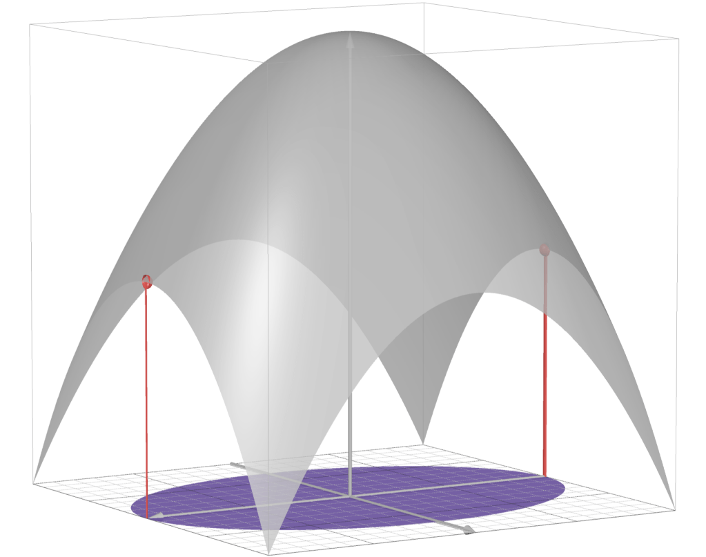
 problem may become analytically solvable or numerically efficient.

 defined in terms of linear equalities/inequalities;
 , or succinctly written
  .
.
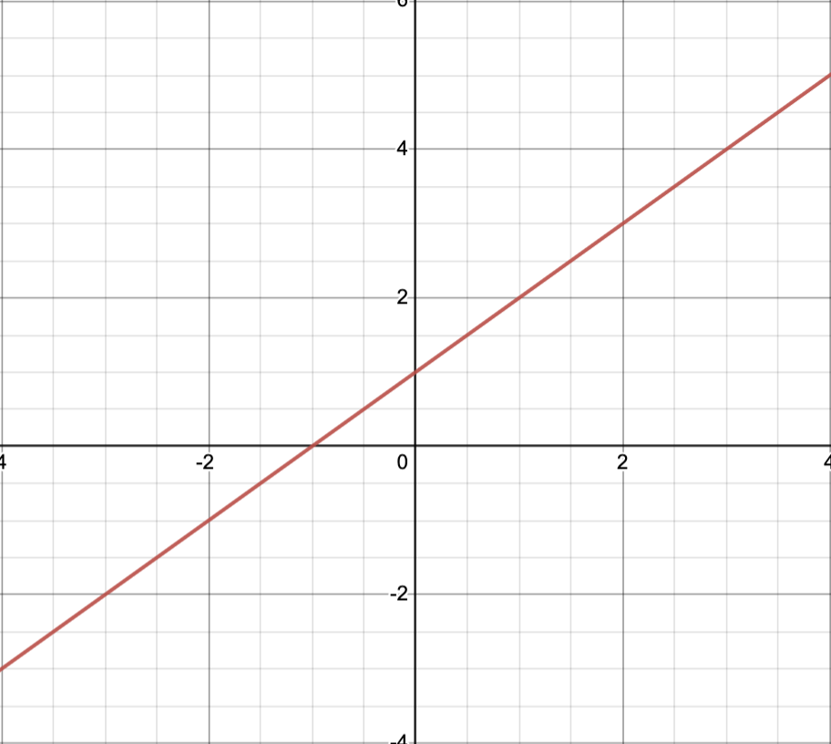


 and
and 
 sparse
 lots of cancellation
 , then


 = transpose of the column vector
  .
. ,
,  , solve

 and
and  .
.
is local minimizer of
for
.)
than any linear function.


is some norm
is the (convex) objective function
are convex.
 ,
,  is the identity matrix, and
  .
.

 .
.
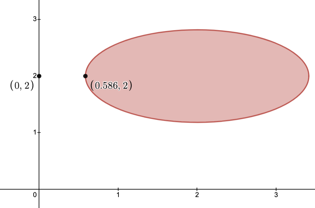
be functions
.
 evolves by

is the time derivative of
are assumed to be given;
;
as an input we are allowed to choose to dictate the evolution
; i.e.,
, the system experiences “feedback.”
so that


 satisfying:

![t \in [0,1]](https://s0.wp.com/latex.php?latex=t+%5Cin+%5B0%2C1%5D&bg=ffffff&fg=111111&s=3&c=20201002)

 contains all line segments whose endpoints belong to
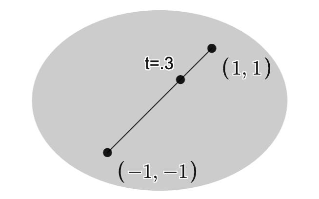
.
and radius
is a convex set.
for all vectors
;
for all vectors
;
iff
.


 be the
  -plane in
  .
.  is affine.
  .)
.)

 is
is

 translated by 3 in the
  -direction:


 and
and  , there holds
  .
.
 .
.
 and
and  belong to
  .
.
 , as desired.
 )
) is a convex cone.
 arbitrary and
  .
.
 with
with  and
and  .
. and
and 
 for
for  since
since  .
.
with normal
,
,
are all convex cones.
if
for
.)
on
,
.


 and scalars
  .
.


 for suitable
  .
.
 satisfying
  ; i.e.,


 satisfying
  for all
  .
. .
. and
and  , then write
  .
.
 is not the same as component-wise inequality, as was the case for vectors.)
 satisfying
  if and only if
  .
. is positive definite, then write
  .
. and
and  , then write
  .
.
 .
. has positive eigenvalues
  , it follows that
  .
.
 iff
iff  .
.
 .
. has nonnegative eigenvalues
  , it follows that
  .
.
 for
for  and so
  .
.
 .
. by showing that
  has positive eigenvalues
  .
.
 ) of this quadratic satisfies
  , from which we conclude the polynomial is positive unless
  and hence
  .
.
 .
.  , either compute its eigenvalues
  or observe that
  and whence
  cannot have only nonnegative eigenvalues.
 is a
is a  -dimensional real vector space and
  is a convex cone in
  and
and  , then it is easy to see:

 .
.
 :
: implies
  , we have the identification

 .
. .
.
 and
and  there holds

 .
. iff
iff


 iff
iff  for all
  .
.
 )
)


 iff
iff  .
.


 )
)


 .)
.)
 was not used anywhere; however,
  immediately implies
  , and
, and  also implies


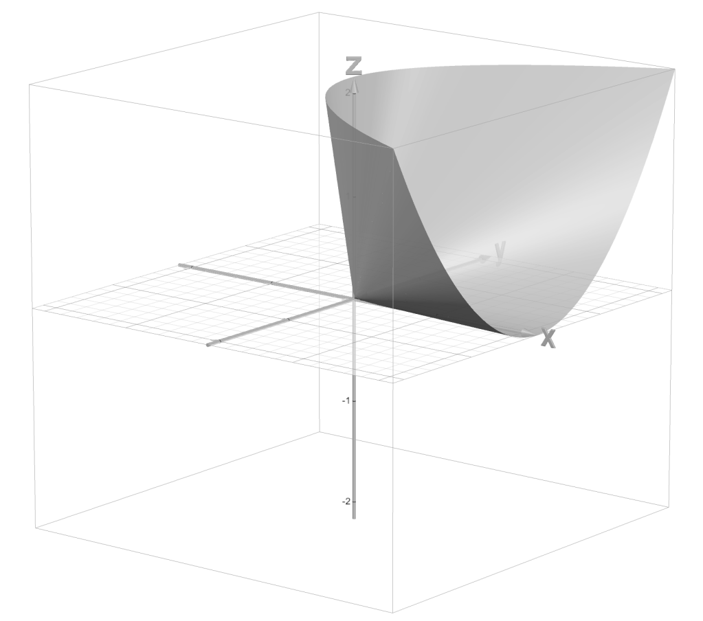
 be two sets.
 and
and  such that

 is said to separate
  into two halfspaces with one containing all of
 separates the pairs
 ![[B,A]](https://s0.wp.com/latex.php?latex=%5BB%2CA%5D+&bg=ffffff&fg=111111&s=3&c=20201002) and
and ![[B,C]](https://s0.wp.com/latex.php?latex=%5BB%2CC%5D+&bg=ffffff&fg=111111&s=3&c=20201002) .
Moreover, the pair
.
Moreover, the pair ![[A,C]](https://s0.wp.com/latex.php?latex=%5BA%2CC%5D+&bg=ffffff&fg=111111&s=3&c=20201002) cannot be separated since
cannot be separated since 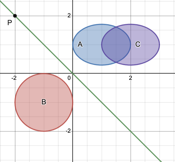

 since neither contain their boundaries.

 with their respective closures
  , the plane
  for
for  and
and  for
for  .
.
 be a fixed set and fix a boundary point


 , then
  is called the supporting hyperplane of
  .
. indicates the closure of
  indicates its interior.)

 .
.
 , we note
  .
. and so

 , showing that
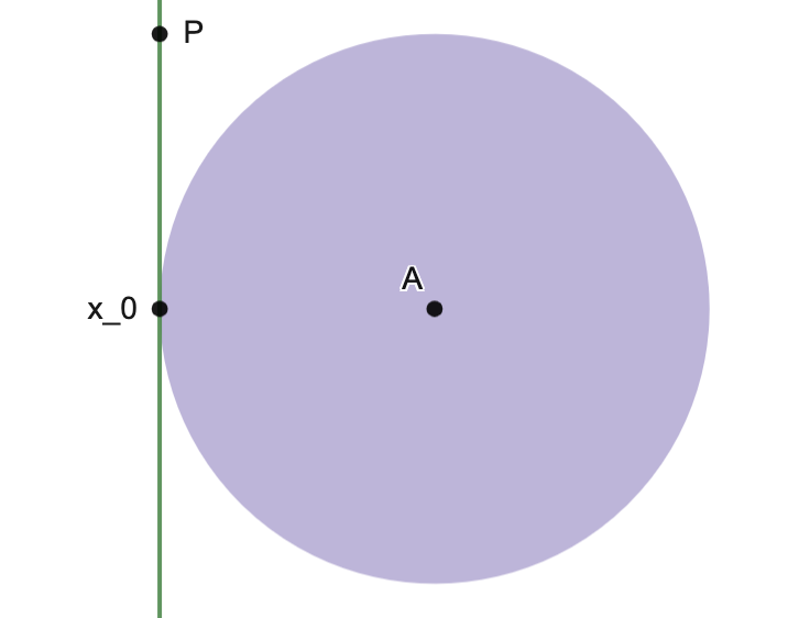

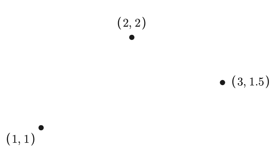
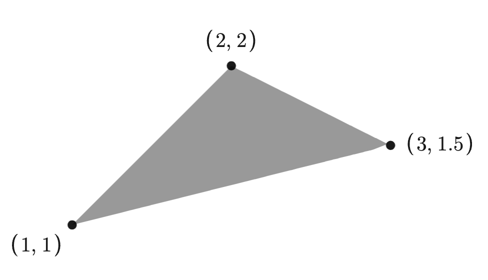

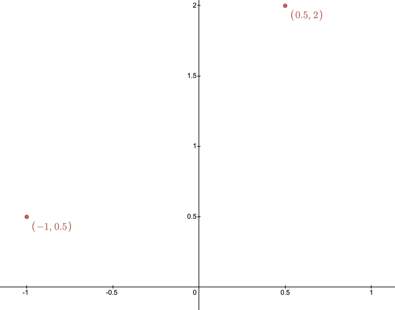
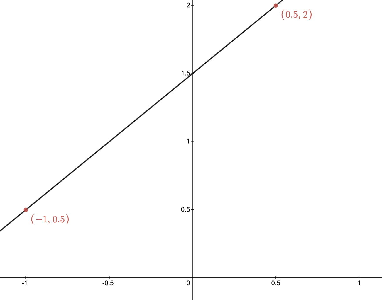

 ,
,  and their conic hull.

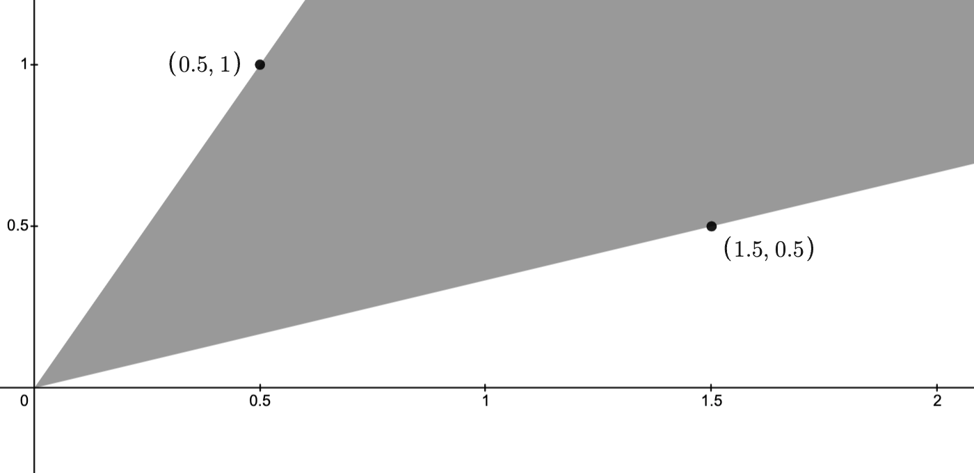
 and
and  , where
 ![t \in [0,1]](https://s0.wp.com/latex.php?latex=t+%5Cin+%5B0%2C1%5D+&bg=ffffff&fg=111111&s=3&c=20201002) and
and  , the conic hull contains all points of the form
  .
.
 and
and  .
.
 satisfying
is closed (i.e.,
.
 on
on 
 is a partial ordering and so
  is not well-defined for all
, then
.
is the standard inequality on
.
, then
.
.
.
depicts those
with
depicts those
, and so
, as indicated in the image.
and
are not comparable.
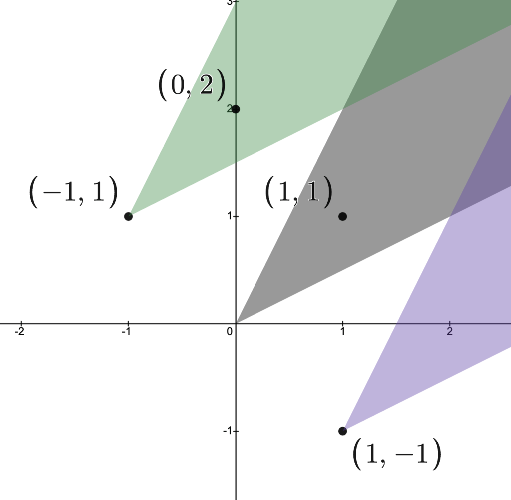

always means a partial function with domain
possibly smaller than
, we may work with the extension
given by
has been extended and to write
and its extension
.
, its indicator function is


 .
.
![x,y \in \text{dom}\, f, t \in [0,1]](https://s0.wp.com/latex.php?latex=x%2Cy+%5Cin+%5Ctext%7Bdom%7D%5C%2C+f%2C+t+%5Cin+%5B0%2C1%5D&bg=ffffff&fg=111111&s=3&c=20201002) there holds
there holds

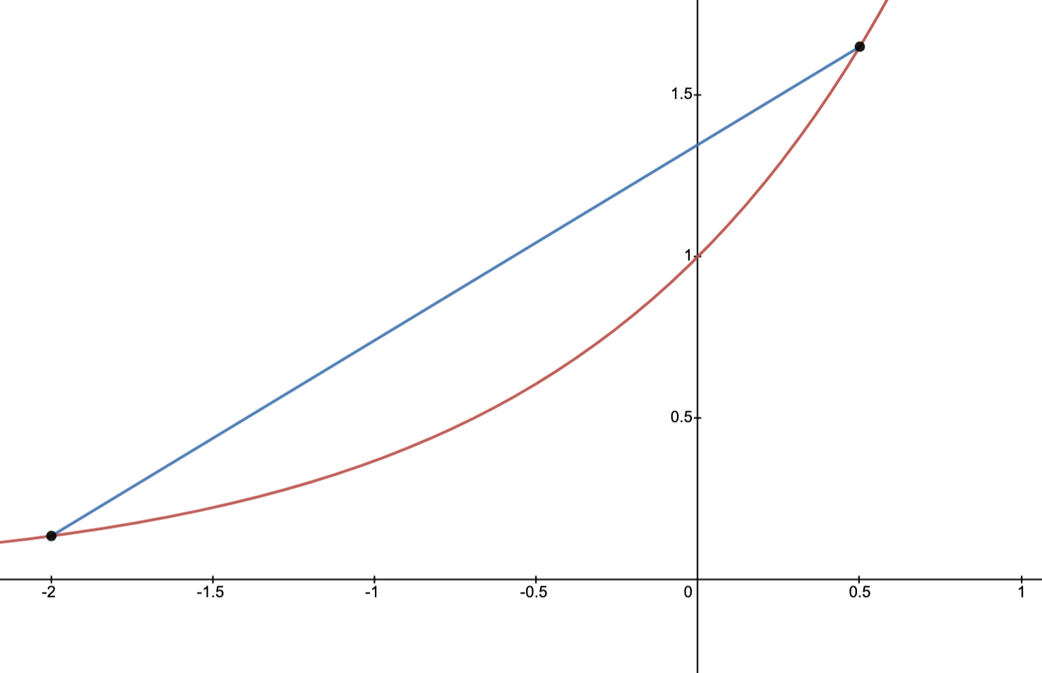
 there holds

 and the dashed line indicates part of the graph of a linear function.

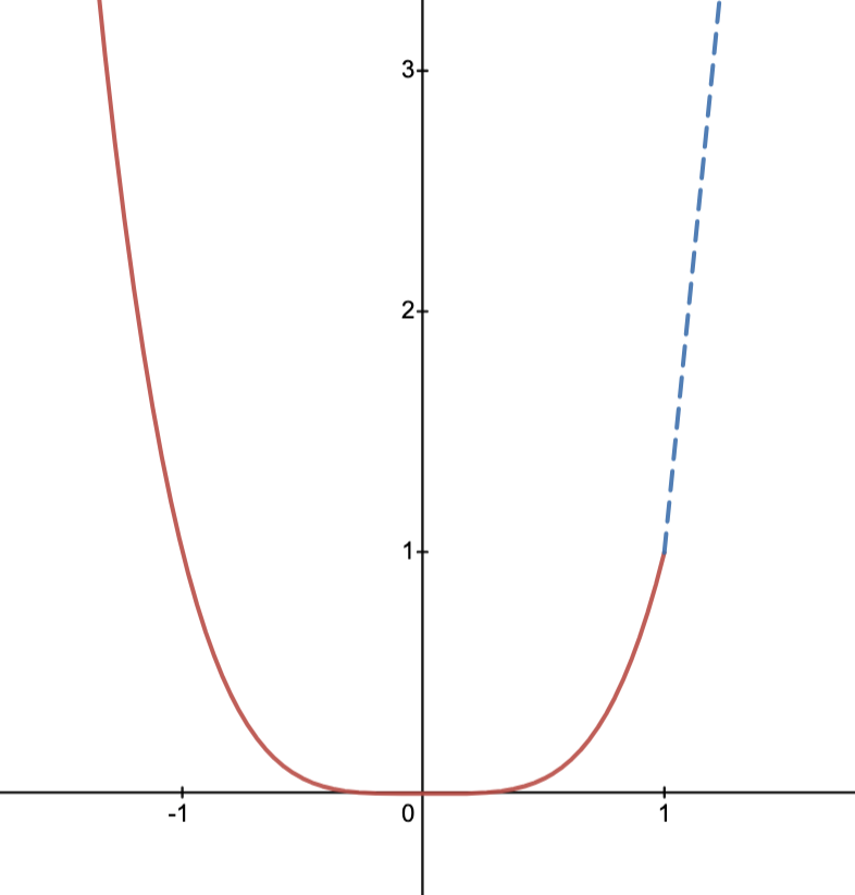
 is, respectively, convex and strictly convex.
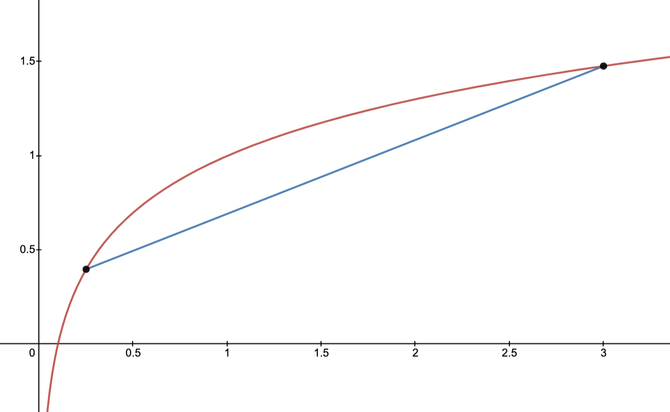
.
is convex in this sense.
to
for any
.


is convex on
.
is convex on
.
is convex on
for
or
and concave for
.
is convex on
is convex (in the extended value sense).

 have convex domain and, given


 by
by


 is convex for all
  and
and  is convex: it is the intersection of
  with the line passing through
  with direction
  .
.
 and
and ![\theta \in [0,1]](https://s0.wp.com/latex.php?latex=%5Ctheta+%5Cin+%5B0%2C1%5D+&bg=ffffff&fg=111111&s=3&c=20201002) and
and  , there holds

 and let
 and
and

 .
.

 ; the higher dimensional case follows by using that

 and add the two inequalities


.
means this hyperplane is a tangent plane at
is just the first order Taylor approximation of


;
;
given by the graph of
.
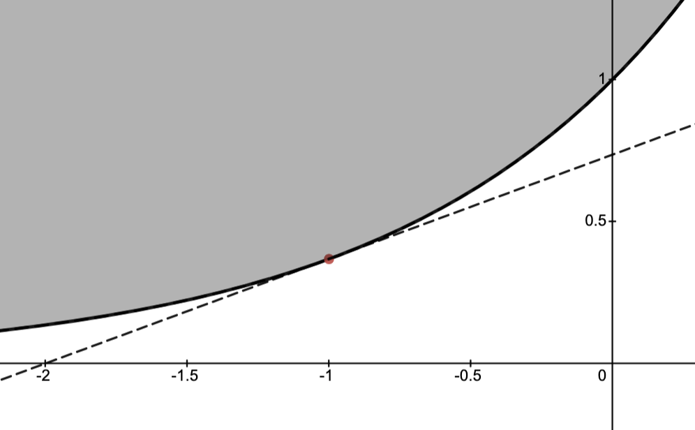
 gives a supporting hyperplane
 is twice-differentiable, then its Hessian is


for all

 -Level set:
 with
with 
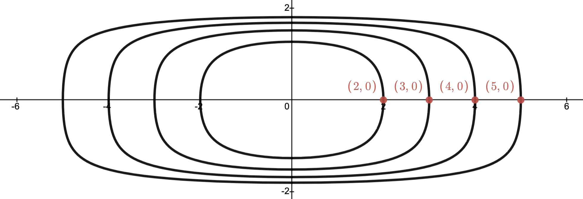

 with
with  .
. for
for  .
.


 for
for 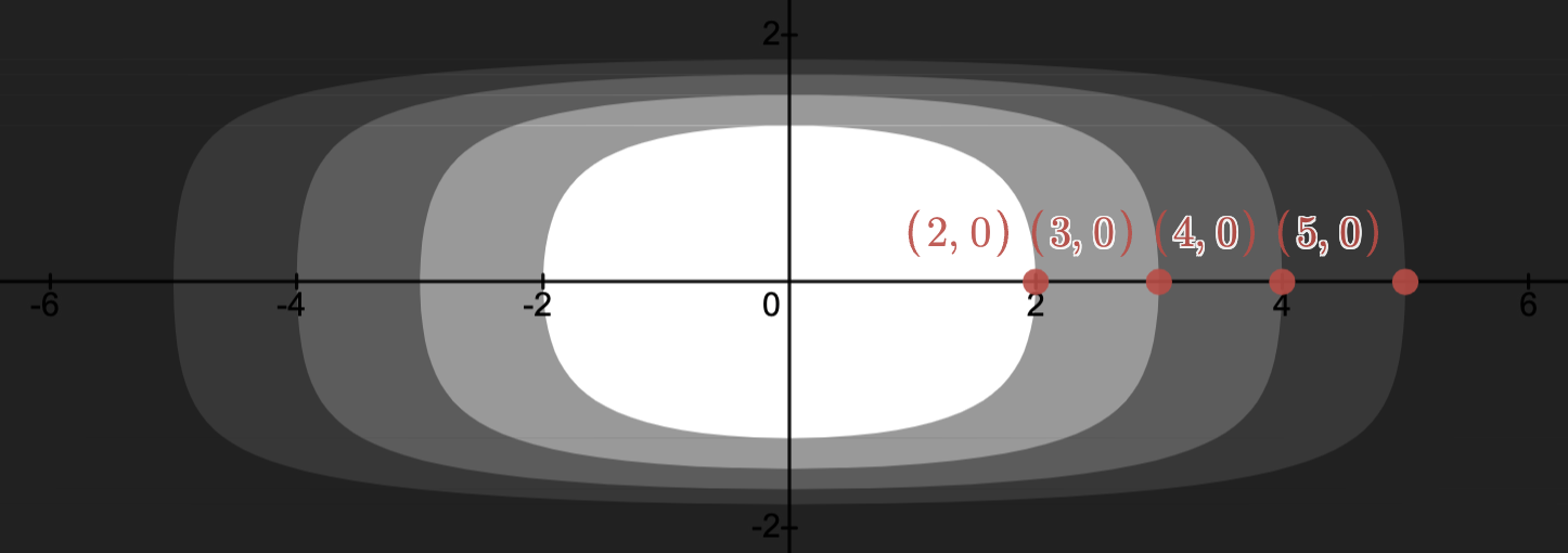
 is convex for all
  is convex for all
  .
.
 implies
  for all
  and so convexity of

 is given below.


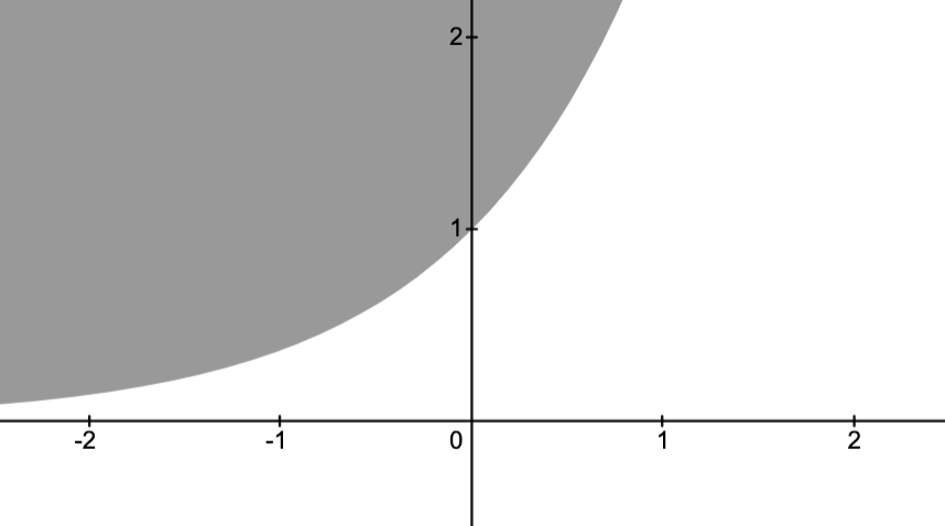

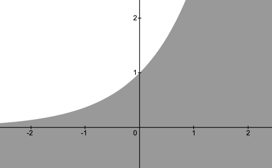
 is convex.
 is convex.
 be distinct points.
 for
for  be the line passing through
  be the two intersection points of
  is in
is in  .)
.) for
for  for
for  .
. is convex.
 .
. for
for 


 is affine and hence convex.


 .
.
 for which
  is bounded above on
  is a differentiable convex function denoting the cost to produce
  , the profit of selling
 is just the optimal profit for selling at price
  .
. is concave for each
  is maximal at
  , i.e., when
  .
. .
. is then given by
  .
. ,
,
is just called the conjugate function of
is the supremum of a family of affine functions,
,
.


 :
: is unbounded on
  since
since


 :
:
 maximizes
  and so

 :
:
 and so


 , it follows that


 .
.
 .
. , then


 .)
.)
 satisfy


 , let
, let


 and let


.
.
.
.
implies
is invertible since then
.


 .
.

 .
. on
on  is convex; equivalently

 be a proper cone and let
  .
.
 and
and 
 and
and  , there holds

.
-convex iff:
and
, there holds
, i.e., iff
is
-convex iff :
.
-convexity is often called matrix convexity.
is convex for all
.


 satisfying

 consisting of the feasible points.
 .
.
 which satisfy the inequality and equality constraints.


 is the feasible set.

as
approaches a point on the circle
, and


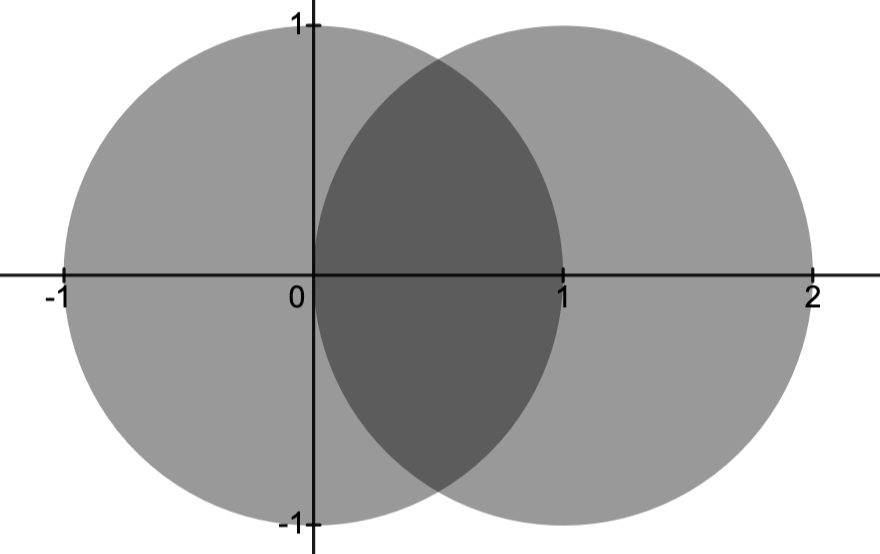

 lies outside of the intersection of the two disks.


 is the largest
  such that
  for all
  .
. .
.
 on
on  .
. .
.
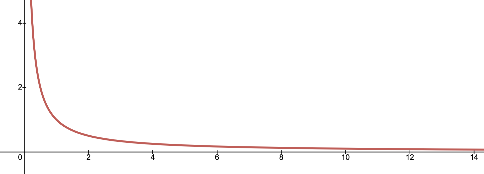


 is attainable.
 .
.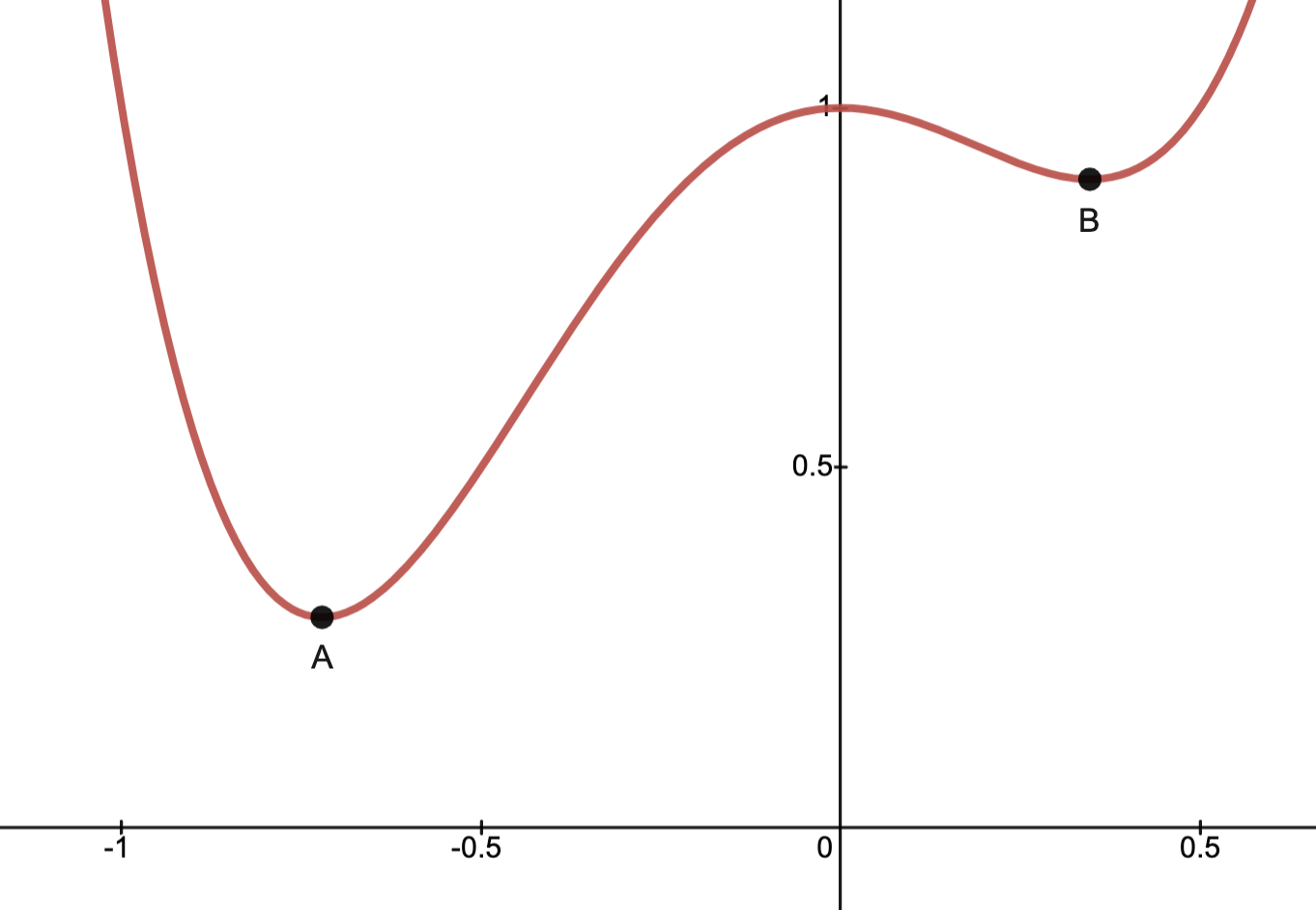
iff the (OP) is solvable.
is not well-defined unless the (OP) is solvable.
if
if the OP is infeasible.


(noting
)
for
for
![\begin{cases} \text{minimize} & f(x) = x^2\\ \text{subject to}& x \in [1,2] \end{cases} \quad \text{and} \quad \begin{cases} \text{minimize}&g(x) = (x+1)^2+1 \\ \text{subject to}&x \in [0,1] \end{cases}.](https://s0.wp.com/latex.php?latex=%5Cbegin%7Bcases%7D+%5Ctext%7Bminimize%7D+%26+f%28x%29+%3D+x%5E2%5C%5C+%5Ctext%7Bsubject+to%7D%26+x+%5Cin+%5B1%2C2%5D+%5Cend%7Bcases%7D++%5Cquad+%5Ctext%7Band%7D+%5Cquad++%5Cbegin%7Bcases%7D+%5Ctext%7Bminimize%7D%26g%28x%29+%3D+%28x%2B1%29%5E2%2B1+%5C%5C+%5Ctext%7Bsubject+to%7D%26x+%5Cin+%5B0%2C1%5D+%5Cend%7Bcases%7D.+&bg=ffffff&fg=111111&s=3&c=20201002)
![x^\star \in [1,2]](https://s0.wp.com/latex.php?latex=x%5E%5Cstar+%5Cin+%5B1%2C2%5D+&bg=ffffff&fg=111111&s=3&c=20201002)

![[1,2]](https://s0.wp.com/latex.php?latex=%5B1%2C2%5D+&bg=ffffff&fg=111111&s=3&c=20201002)
![x^\star - 1 \in [0,1]](https://s0.wp.com/latex.php?latex=x%5E%5Cstar+-+1+%5Cin+%5B0%2C1%5D+&bg=ffffff&fg=111111&s=3&c=20201002)

![[0,1]](https://s0.wp.com/latex.php?latex=%5B0%2C1%5D+&bg=ffffff&fg=111111&s=3&c=20201002)
 to the first problem, we readily obtain the solution
  to the second problem, and vice versa.
 is an injective function with
  .
. , we have


solves (OP2).
such that
solves (OP2).)
solves (OP1).

 .
.
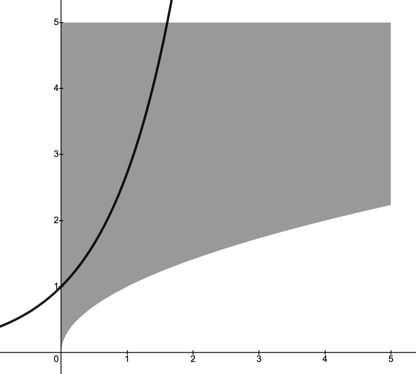


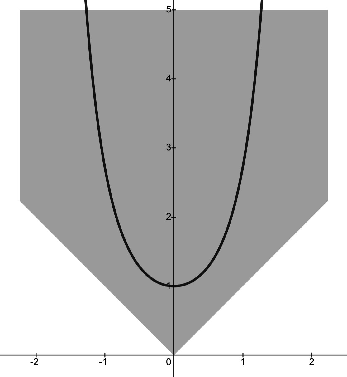
 be such that
  .
. for some
  .
.


 many variables.
(Recall:
many variables.
(Recall:  .)
.)
with
solves (OP2), and
solves (OP1)

 .
.

 , and so


 with optimal value
  .
.

 , then there is a variable
  such that
  ; such a variable
  is called a slack variable.
 , the problem


be the feasible set of (OP1) and
that of (OP2).
and
; i.e., the feasible sets are not the same object.
and the paraboloid-type set depicts the feasible set
with slack variable
.

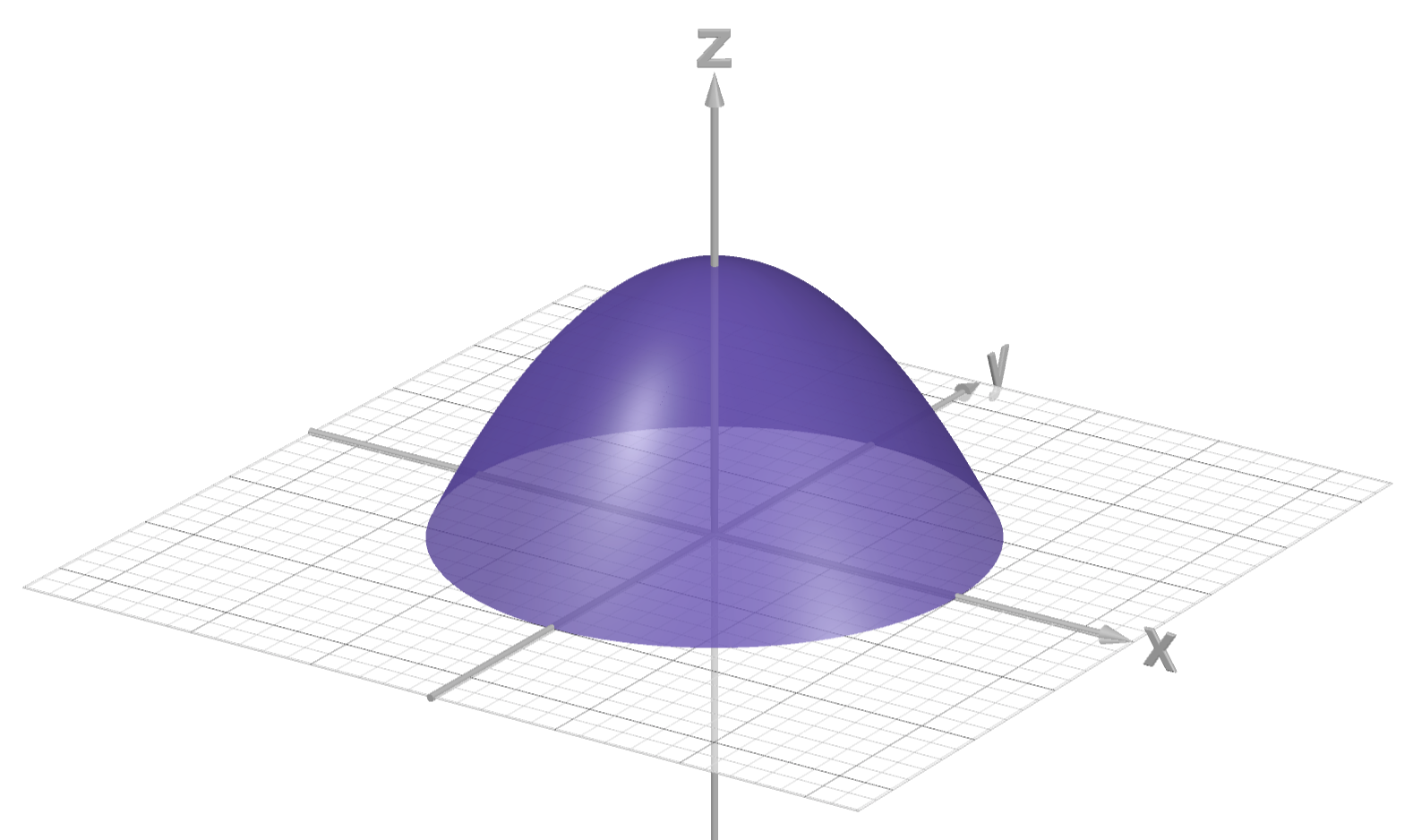

 may be easier than solving the system of inequalities


 satisfying


 is just a matter of solving a system of equations and choosing those
  with
with 
 .
.
 subject to constraints is equivalent to finding the smallest
  for some feasible
  .
. for different values of
  for which
  is given by
  .
.
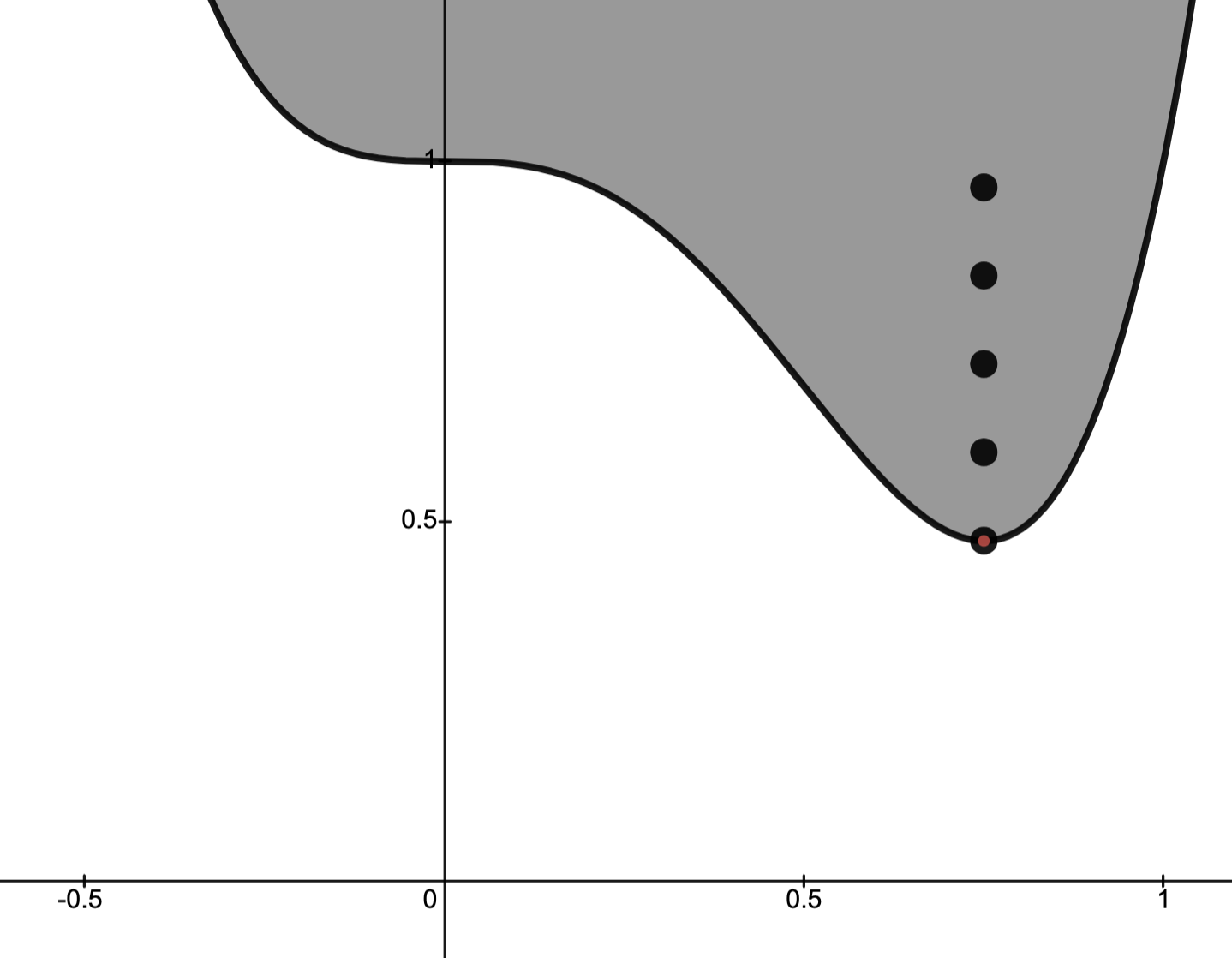
 and sets
  with
with  let
let


 for any real number
  .)
.)
 , one may instead minimize
  and then take the minimum optimal value of this procedure.
 and where the feasible set
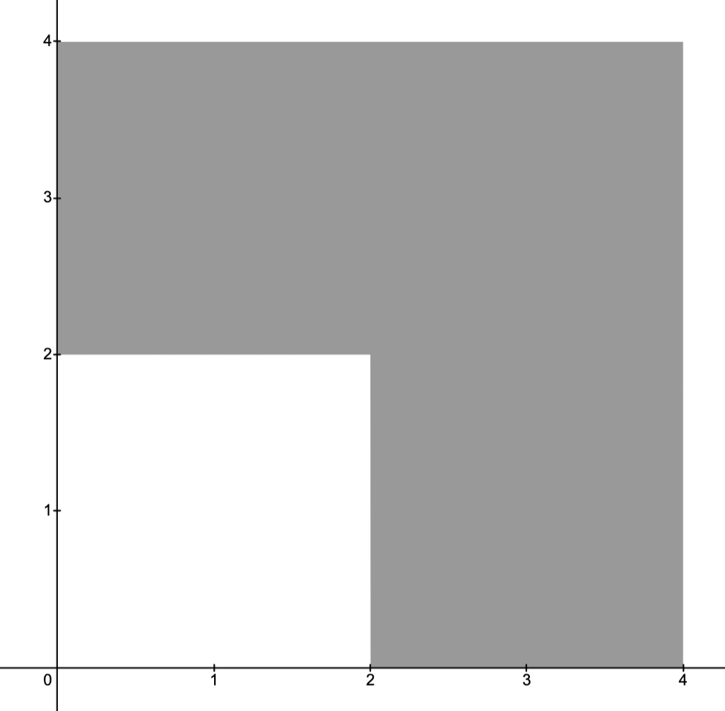
 as indicated below.
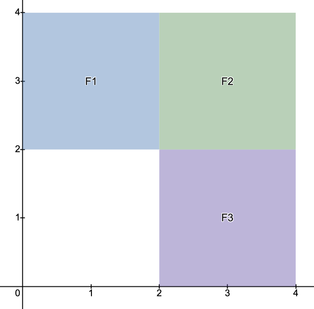

 , and let
  be the optimal value for (OPi).

and
are fixed.


 is quasilinear, then
  defines a convex set.
 convex does not imply the level set
  gives a sphere.

 and that there is a
  such that

 for all
  with a distance at most
  of
of  such that
  .
. .
.


 , there holds


 there holds


 , noting that
  since
since 
 in the direction
  and so
  for small
  defines a line passing through
  , it follows that
  is the directional derivative in direction
  , i.e.,
  .
.


 (equivalently, there are no nontrivial constraints),
  is a minimizer iff


 .
.
 is open and so, for small

 iff
iff 

 implies
 .
.is the unique solution to (OP);
and
has an affine set of solutions.


 is a minimizer iff

 .
.is an inconsistent system
,
for some
.


 is a linear space, this is only possible iff


 and so this condition means there exists
  such that


 ):
): the vector inequality


 satisfying the matrix inequality
  , which means
  is positive semidefinite.
 ,
,  , then

 , then

 )
)


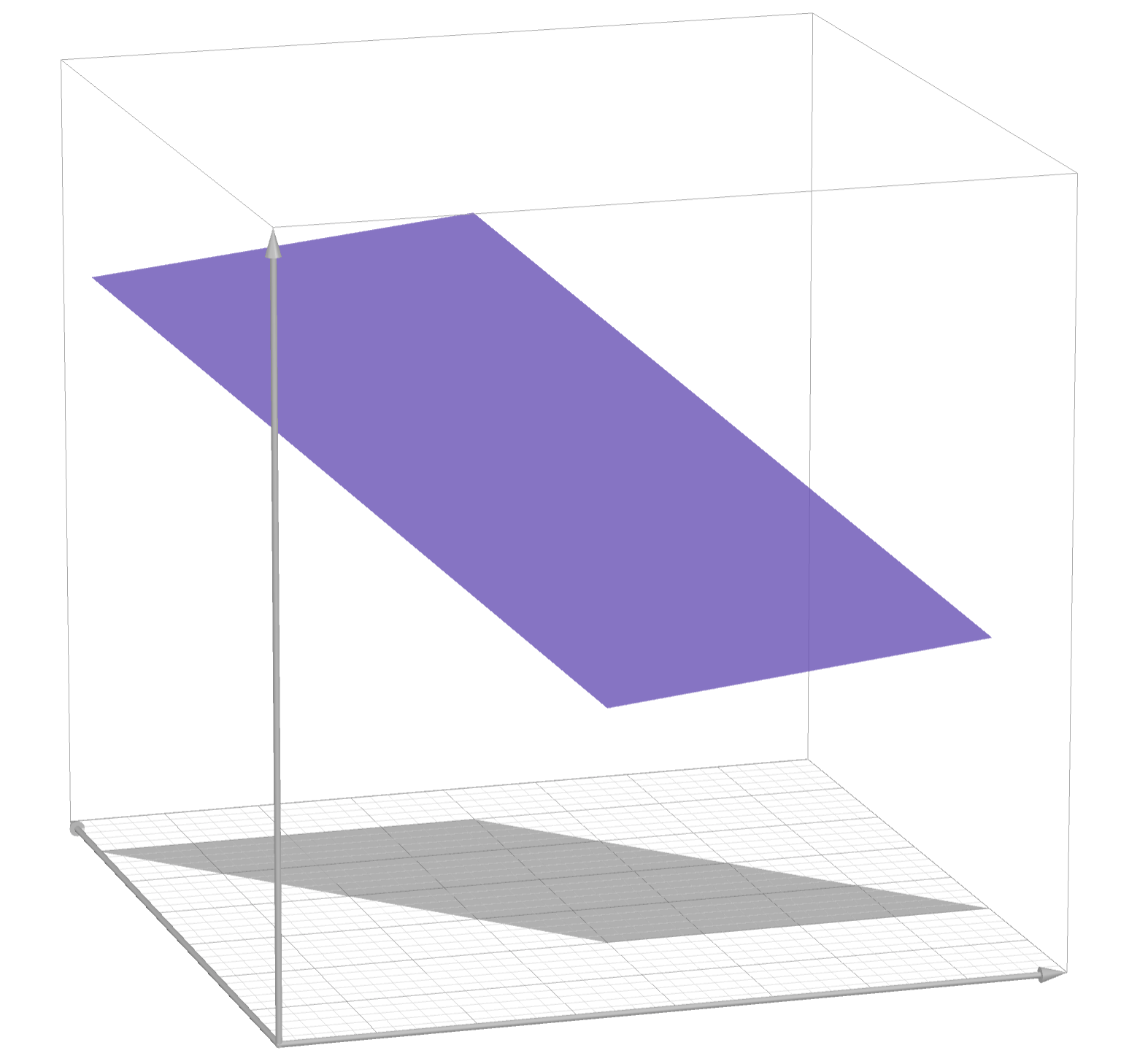
, have equivalent problem with objective
.
to solve problem.
over a polyhedron a (LP).


 is suitable for parameters which take on discrete quantities.

 satisfying

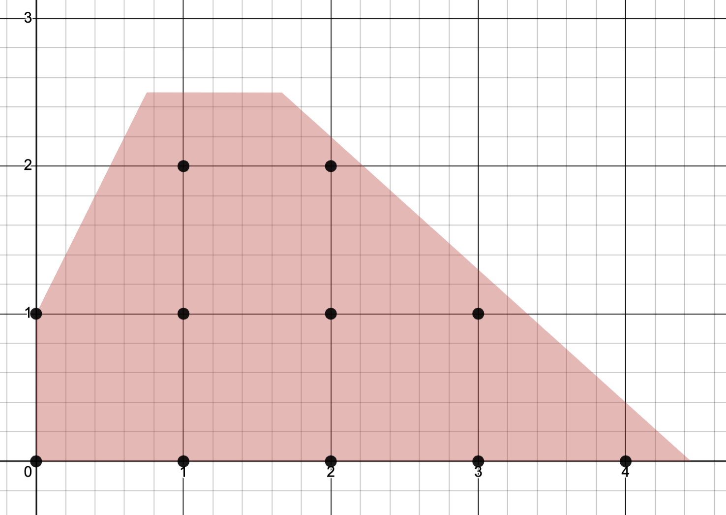
, then the problem is called a boolean linear program:
instead.


.
solves the (LP), then it solves the (ILP).


![F \to \{x \in [0,1]^n: Gx \preceq h \}](https://s0.wp.com/latex.php?latex=F+%5Cto+%5C%7Bx+%5Cin+%5B0%2C1%5D%5En%3A+Gx+%5Cpreceq+h+%5C%7D+&bg=ffffff&fg=111111&s=3&c=20201002)

 workers and
  locations with
  ,
,


 .
. are binary is of course natural for the problem.
 since the
  th location not operating means it cannot host a worker; thus we have
  .
.
![\begin{cases} \text{minimize} & c^Tx + \text{tr}\,(C^TX)\\ \text{subject to} & x \in [0,1]^n\\ &X \in [0,1]^{m \times n}\\ &\sum_{j=1}^n x_{ij} =1, i = 1,\ldots,m\\ & x_{ij} \leq x_j, i=1,\ldots,m,j=1,\ldots,n \end{cases}.](https://s0.wp.com/latex.php?latex=%5Cbegin%7Bcases%7D+%5Ctext%7Bminimize%7D+%26+c%5ETx+%2B+%5Ctext%7Btr%7D%5C%2C%28C%5ETX%29%5C%5C+%5Ctext%7Bsubject+to%7D+%26+x+%5Cin+%5B0%2C1%5D%5En%5C%5C+%26X+%5Cin+%5B0%2C1%5D%5E%7Bm+%5Ctimes+n%7D%5C%5C+%26%5Csum_%7Bj%3D1%7D%5En+x_%7Bij%7D+%3D1%2C+i+%3D+1%2C%5Cldots%2Cm%5C%5C+%26+x_%7Bij%7D+%5Cleq+x_j%2C+i%3D1%2C%5Cldots%2Cm%2Cj%3D1%2C%5Cldots%2Cn+%5Cend%7Bcases%7D.+&bg=ffffff&fg=111111&s=3&c=20201002)


 , then the problem is convex (see remarks).
,
implies
is just a convenient normalization.
ensures the (QCQP) is convex.
, respectively.
(i.e.,
) is not a serious restriction.
is a scalar, we have
.
.
.
:
.
with
.


 and
and  .
..
,
is the pseudo-inverse (aka Moore-Penrose inverse) of
.
 )
) means the vector norm


 is equivalent to a (LS) problem with matrix of size
  .
., where “best” is chosen to mean in terms of the vector norm
is equivalent to minimizing
ensures
is not differentiable at
, but
is.)


 , observe:
and so
, i.e.,
is symmetric;
,
.

 iff
iff

iff
.


 be convex subsets.
 , which pair
  ?
?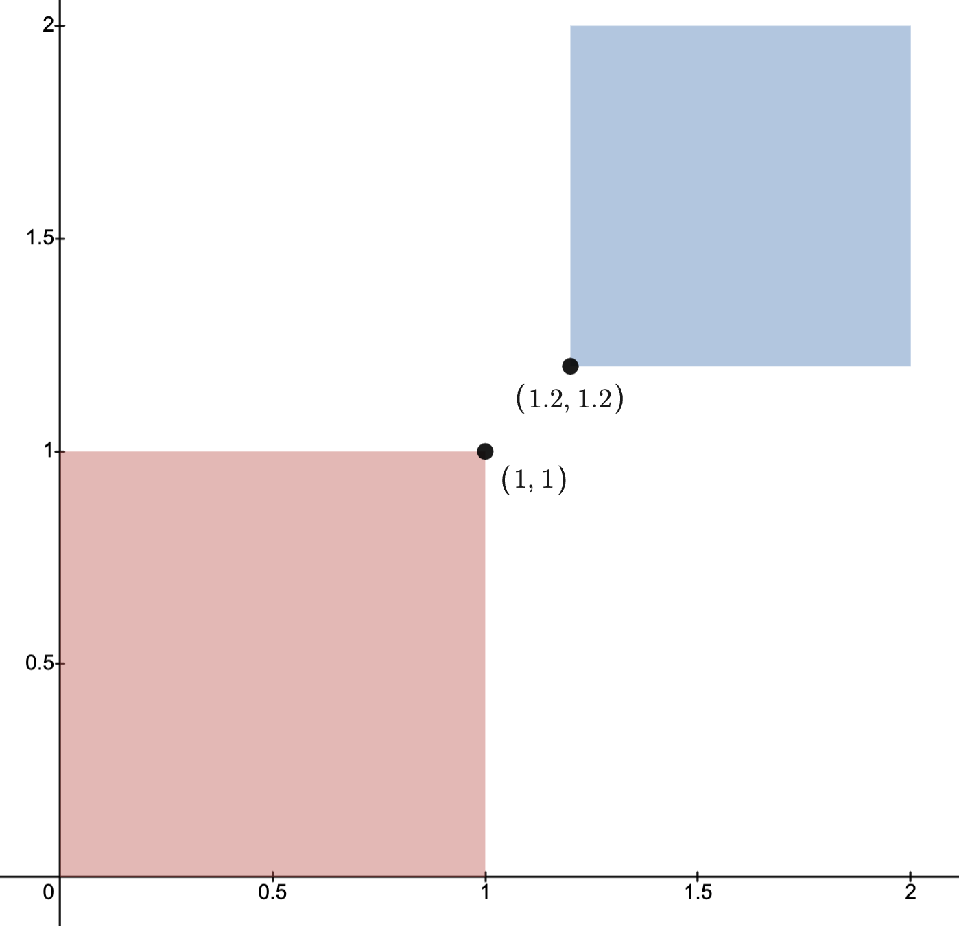

 convex, then the (NPP) for
  is the (COP)


 iff
iff 


 be polyhedral domains such that

![[P_1,P_2]](https://s0.wp.com/latex.php?latex=%5BP_1%2CP_2%5D+&bg=ffffff&fg=111111&s=3&c=20201002) and
and ![[Q_1,Q_2]](https://s0.wp.com/latex.php?latex=%5BQ_1%2CQ_2%5D+&bg=ffffff&fg=111111&s=3&c=20201002) provide (QP) relaxations of the (NPP) for
provide (QP) relaxations of the (NPP) for ![[K_1,K_2]](https://s0.wp.com/latex.php?latex=%5BK_1%2CK_2%5D+&bg=ffffff&fg=111111&s=3&c=20201002) and, respectively, provide upper and lower bounds for the optimal values for the original (NPP).
and, respectively, provide upper and lower bounds for the optimal values for the original (NPP).


.
is a group and
a “conic representation” of


 ).
). to mean the change of variable given by

 convex function)
 :
:


 is convex since affine functions are convex.
 , let
, let


is too weak to break the convexity of
and
.


 .
.


 , we write
  to mean
  for all
  .
.


 , we conclude


 , define


 are the components of


choice of domain (a halfspace) of objective and ensures convexity.
concave problem.


 , then

 , we have


 iff
iff


 matrices


 and
and  .
.


 satisfying


and
be arbitrary.
and for arbitrary
.
is a lower bound of


 , then


 is an underestimater of the objective function


 , the problem


 is convex.


 .
.


.
iff
.


 satisfy


 , there holds


 :
:


 , among all (closed) origin centered ellipsoids
  satisfying
  , find those with minimal volume.
 , the set

 is proportional to
  .
. for some
  implies

 .
. gives the ball of radius
  .
.
 satisfying
  which minimize
  is convex, and so we may reformulate the problem as the following (COP):

for
;
with vector
;
.
 , noting
  .
.


 is
is

 provides a lower bound of the optimal value, we conclude: if
  is the optimal volume, then, up to known constant
  , there holds


 , observe

 , we identify


.
.
is infimum of family of concave functions.
is convex.
minimizing convex
is convex constraint:
to dual are called dual optimal.


 , the Lagrangian for (OP2) is

 is unbounded below if
  .
. , then


 is bounded below.)


 is bounded below iff
  .
.


 .
.


 .
. .
. .
.is possible.


 denote the relative interior of
  means
means  such that


 is feasible but not strictly feasible.
.
are affine and
are not, then it is enough if there holds the weakened Slater condition: there exists a
.

 be the domain.
 .
. ,
,


-plane.
centered at a point in
still lies in
is the shaded region of the ellipse excluding the curve bounding the domain.
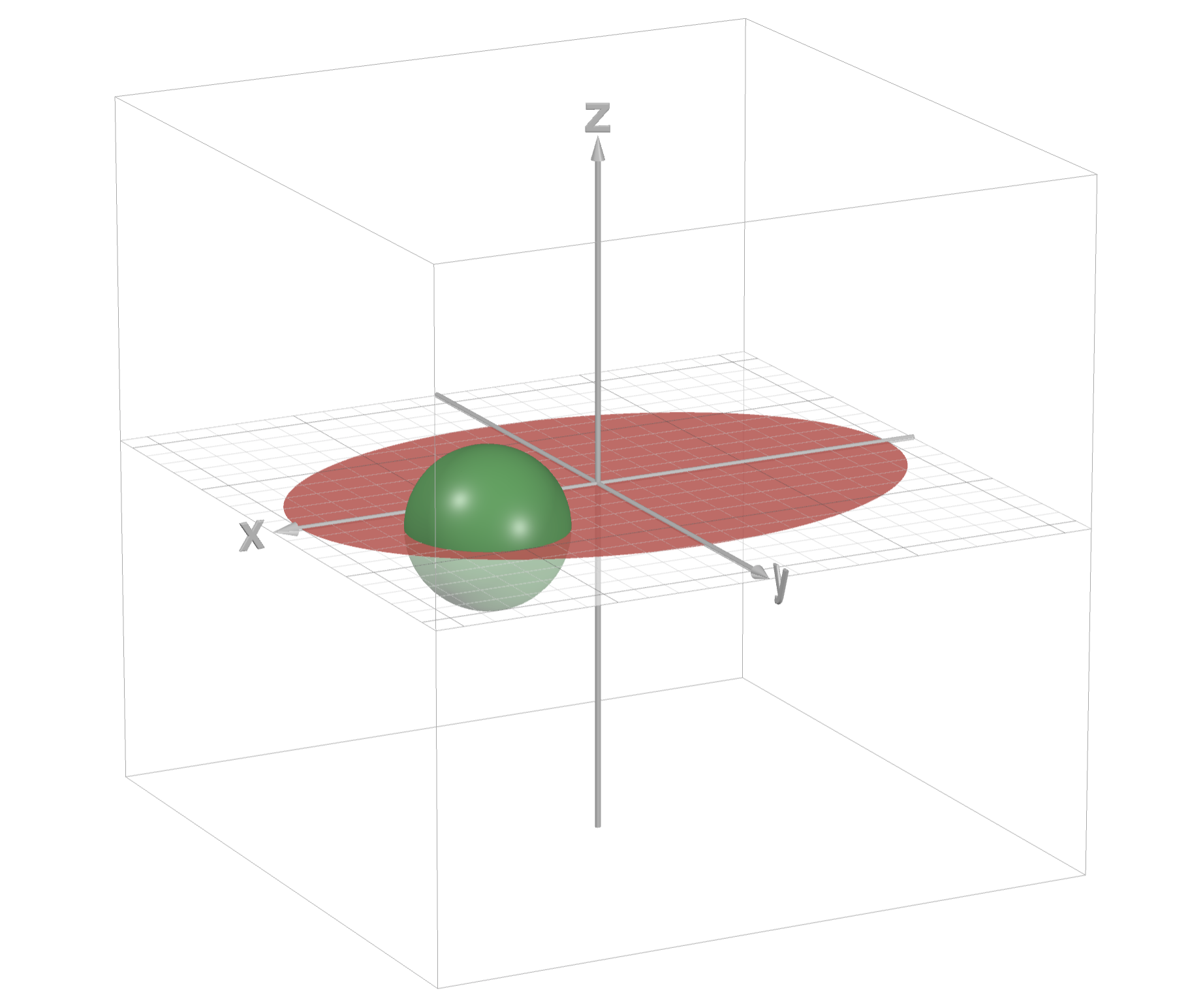
 such that


 are convex.
describes a cube:
,


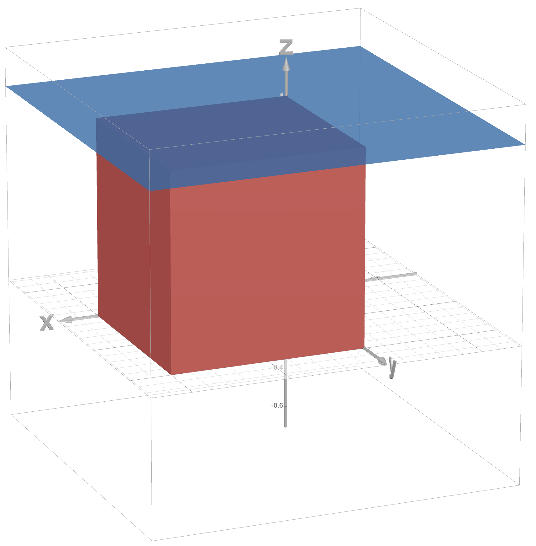
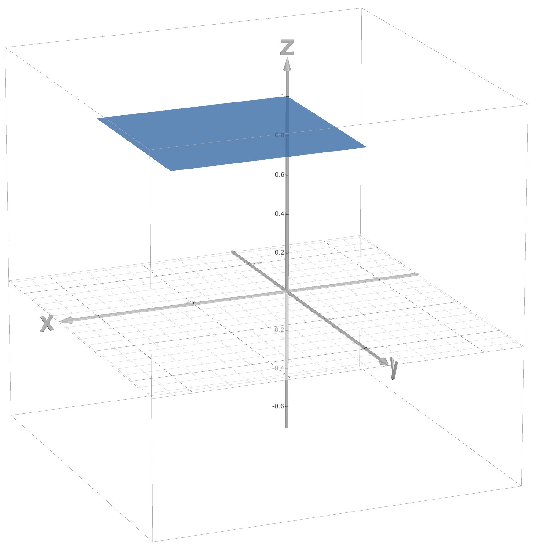
 and (COP) fails Slater’s condition:


 .
. , we see (COP1) satisfies Slater’s condition.
 and
and  be the Lagrangian for (COP) and (COP1) respectively.

might not even be differentiable, in which the KKT conditions for (COP) would be ill-posed.
or
, then the problem fails Slater’s condition.


 .
.
 ):
): .
.

 ):
): .
.
 and
and  .
. .)
.)
 , and so
  .
. .
.


 .
.


 .
. is invertible and
 .
.

 iff
iff


 .
.

 ;
;.
feasible, then
at a feasible pair
, then
,
.
-suboptimal without even knowing the primal optimal
with
at worst
.
in search of optimal
.
gives feasible
within allowed error:
.
.
is dual optimal, then
.
and
, we have
is permissible.
,
, we conclude
and
, the sum

![p^\star,d^\star \in [g(\lambda,\nu),f_0(x)]](https://s0.wp.com/latex.php?latex=p%5E%5Cstar%2Cd%5E%5Cstar+%5Cin+%5Bg%28%5Clambda%2C%5Cnu%29%2Cf_0%28x%29%5D+&bg=ffffff&fg=111111&s=3&c=20201002)


 are differentiable and have open domains.
 are optimal with zero optimality gap, then

 ,
, 

 with dual optimal Lagrange multipliers.
 is differentiable and
 or
or  are zero.


 satisfy the KKT conditions, then they automatically primal and dual optimal, respectively.


 is dual feasible since


 vanishes and hence
 implies


 and
and  is the vector of 1’s.
.
.
with
and so (WF) satisfies strong duality.


 if it satisfies the system of equations


 is acting as a slack variable.)

 in terms of
  by considering two cases.
 .
.
 if
if  .
.
 .
.
 , then

 .
. .
.


 and hence
 .
.![\begin{aligned} \text{on }[0,\alpha_1] \text{ there holds }& G(t)=0\\ \text{on }[\alpha_1,\alpha_2] \text{ there holds }& G(t) = t-\alpha_1\\ \text{on }[\alpha_2,\alpha_3] \text{ there holds }& G(t) = t-\alpha_1 + t-\alpha_2 = 2t - \alpha_1 - \alpha_2 \end{aligned}](https://s0.wp.com/latex.php?latex=%5Cbegin%7Baligned%7D+%5Ctext%7Bon+%7D%5B0%2C%5Calpha_1%5D+%5Ctext%7B+there+holds+%7D%26+G%28t%29%3D0%5C%5C+%5Ctext%7Bon+%7D%5B%5Calpha_1%2C%5Calpha_2%5D+%5Ctext%7B+there+holds+%7D%26+G%28t%29+%3D+t-%5Calpha_1%5C%5C+%5Ctext%7Bon+%7D%5B%5Calpha_2%2C%5Calpha_3%5D+%5Ctext%7B+there+holds+%7D%26+G%28t%29+%3D+t-%5Calpha_1+%2B+t-%5Calpha_2+%3D+2t+-+%5Calpha_1+-+%5Calpha_2+%5Cend%7Baligned%7D+&bg=ffffff&fg=111111&s=3&c=20201002)
 is continuous.
 is an increasing continuous piecewise linear function.
 may be solved by finding when the graph of
  .
.

 ,
,  , consider the perturbed problem

results in
;
results in relaxing
;
results in tightening
results in “translating” solution set of
.
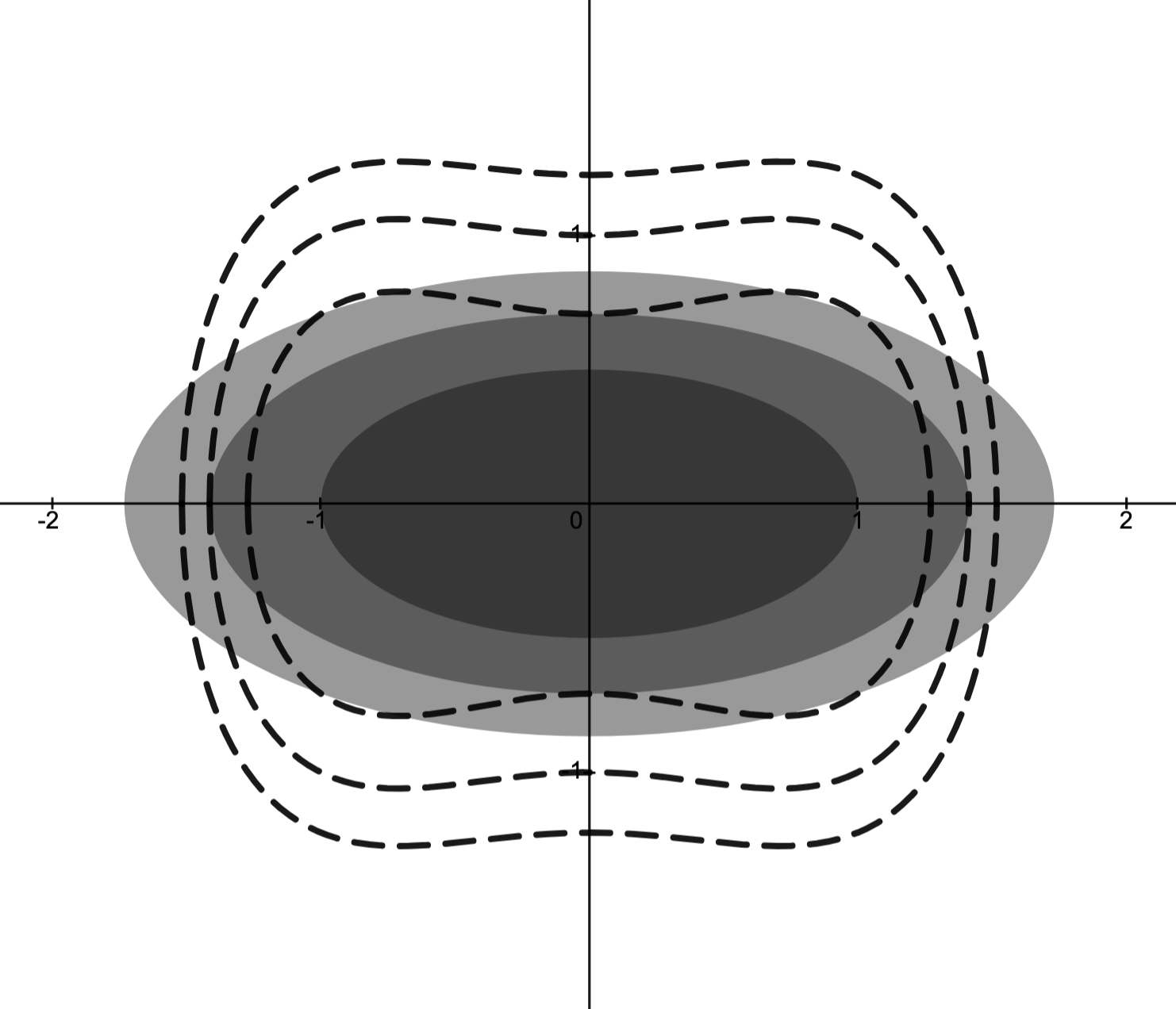

 , respectively.

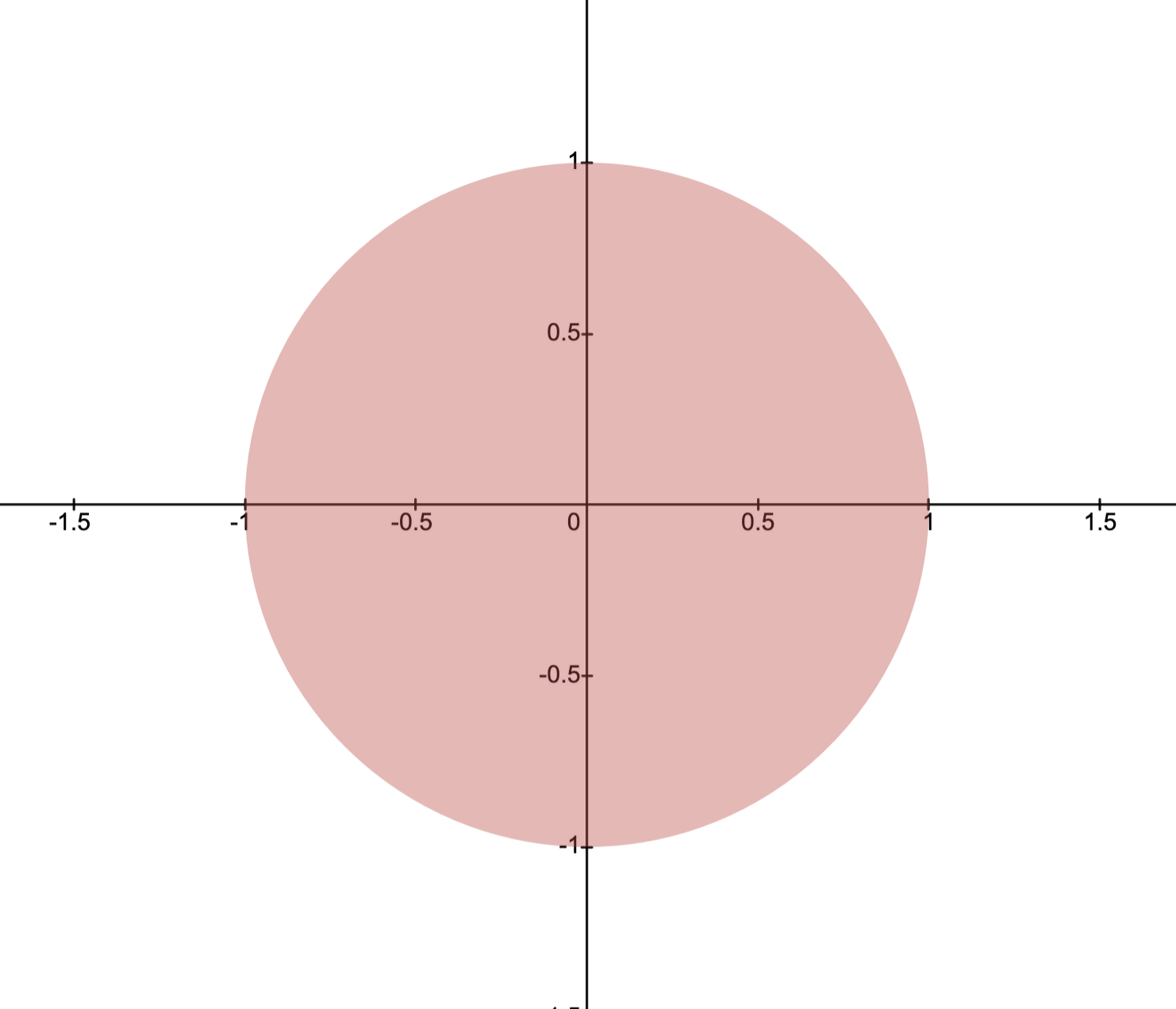
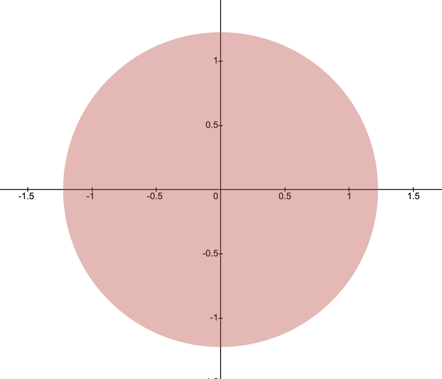

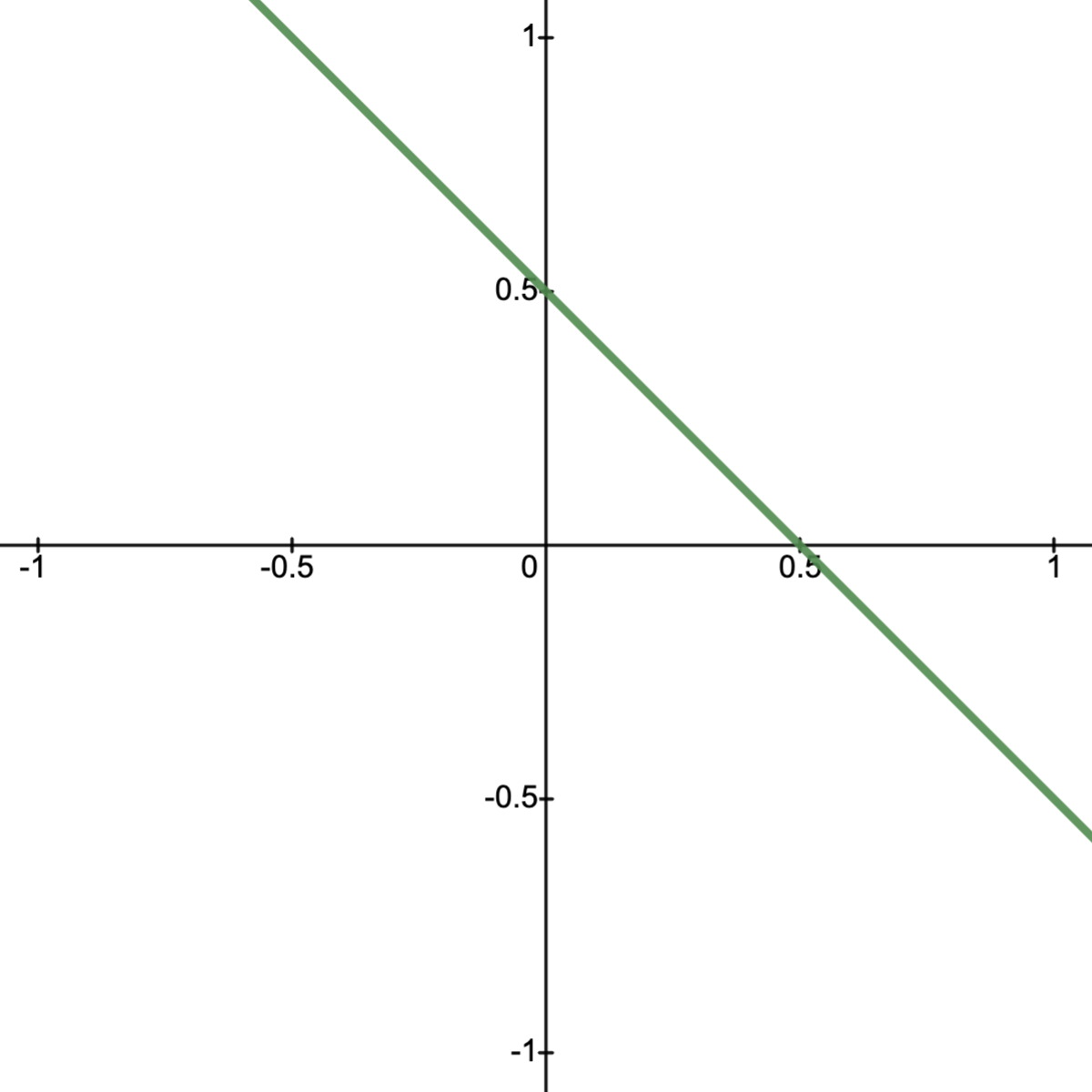
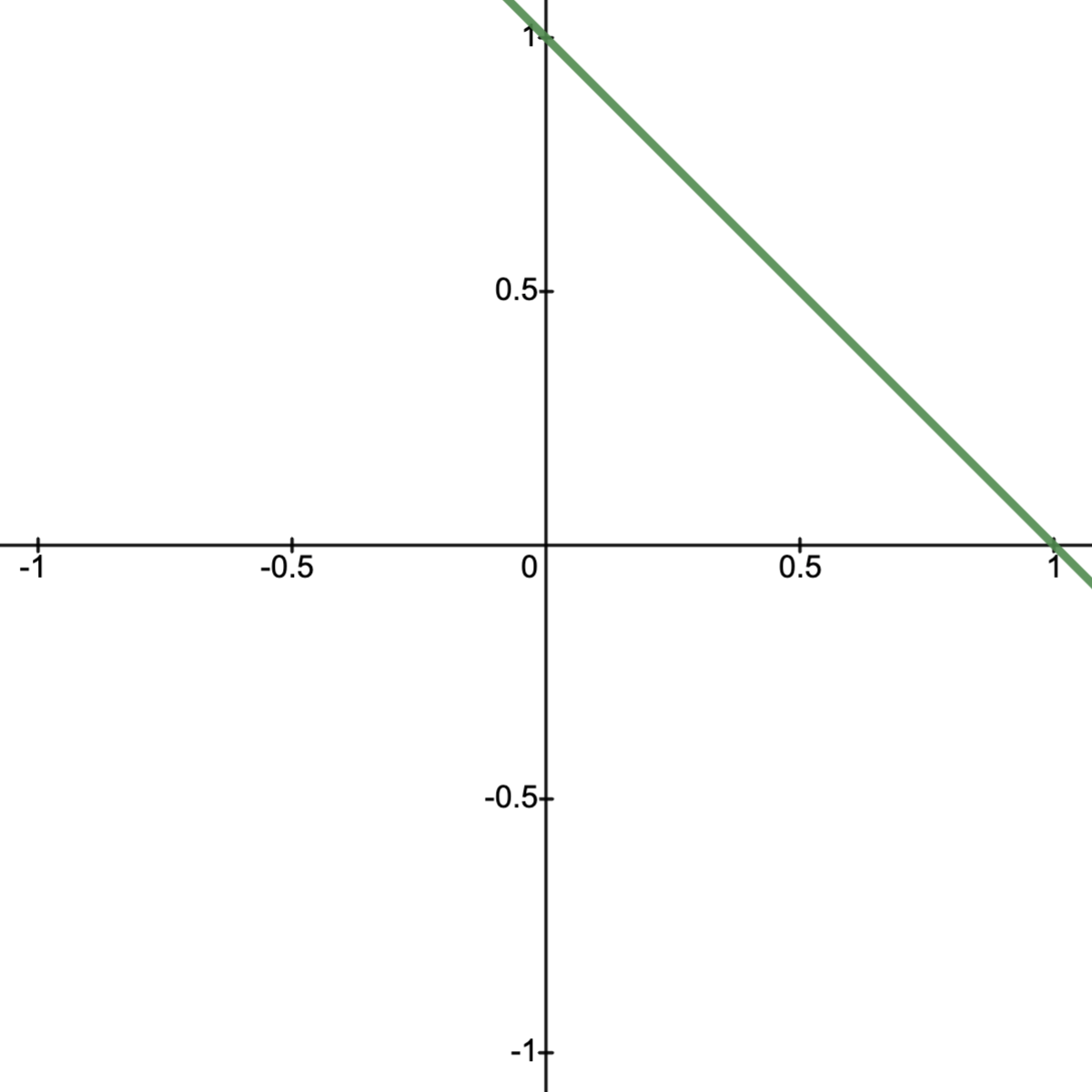
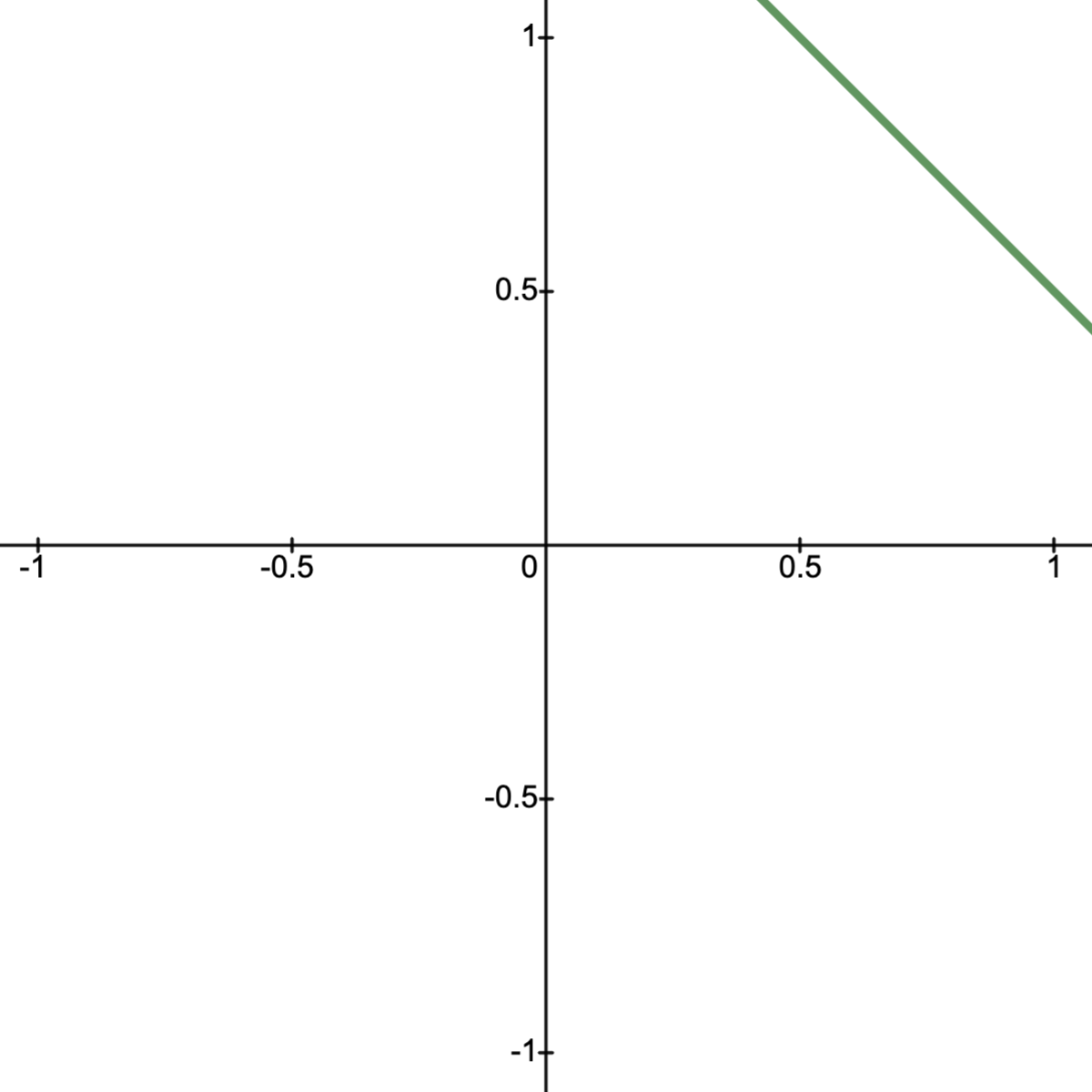
 denote the primal optimal value for
  .
.
 the primal optimal value
 primal optimal value of unperturbed problem;
, then the perturbation
, then the perturbation

 and the constraint, problem is:

![[0,1]](https://s0.wp.com/latex.php?latex=%5B0%2C1%5D&bg=ffffff&fg=111111&s=3&c=20201002)


![[0,1+u]](https://s0.wp.com/latex.php?latex=%5B0%2C1%2Bu%5D&bg=ffffff&fg=111111&s=3&c=20201002)


 is plotted below; observe the behavior of
  as the constraint is relaxed.
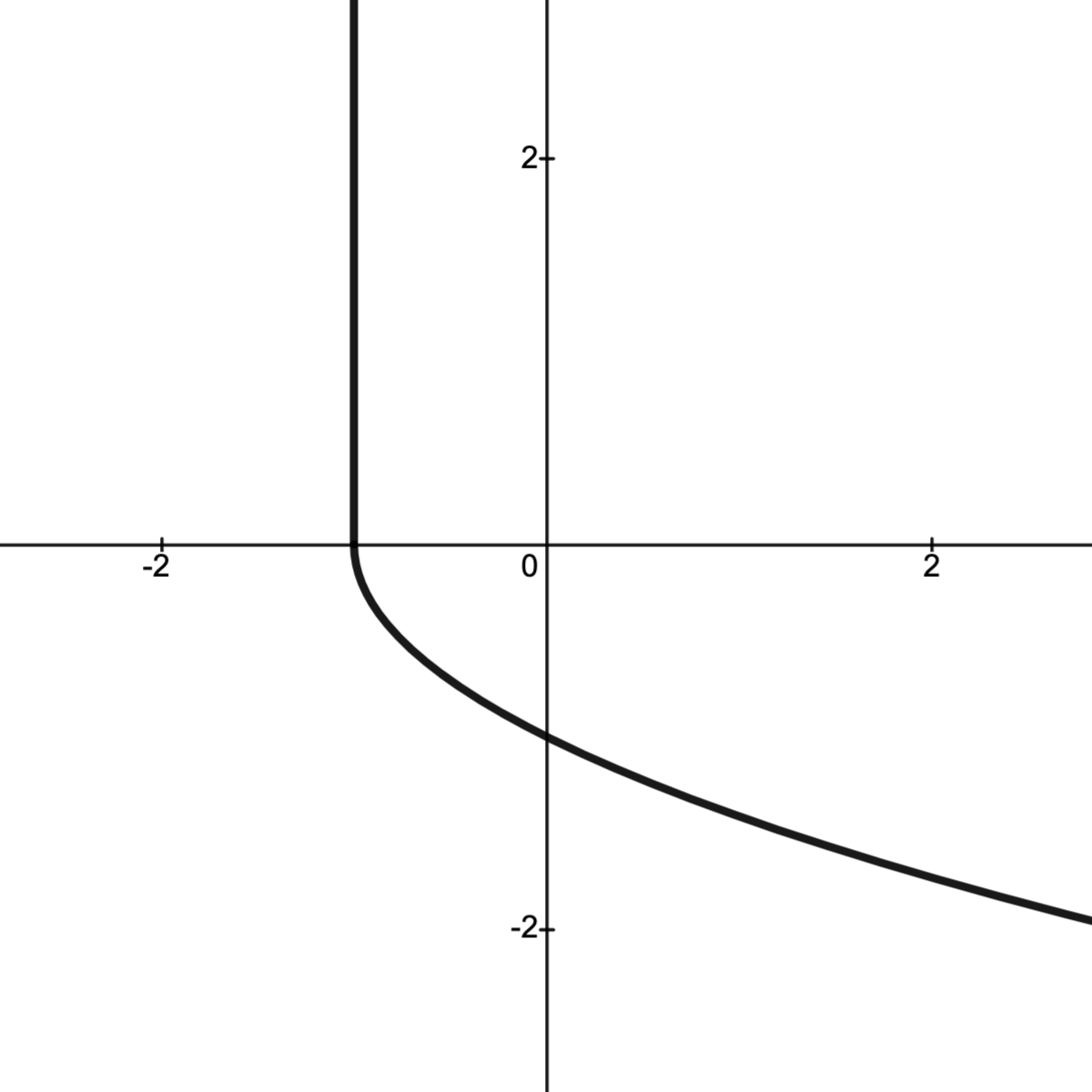
 is achieved by dual feasible
 and let


 may determine the sensitivity of the primal optimal value subjected to perturbation.

results in increasing
:
without decreasing
too much.
:
: the larger
increases
:
: the smaller
:


 .
.


 , and whence
  , respectively.
 and
and  gives
gives

 .
. is not optimal.
 gives
gives

 .
.


more and more negative.
!
.
.


 iff
iff


 is the smallest
  .
.
 can take among feasible
  .
.
describes a parametric curve in
.
of

corresponds to the portion of
is the dashed line in the graph below.
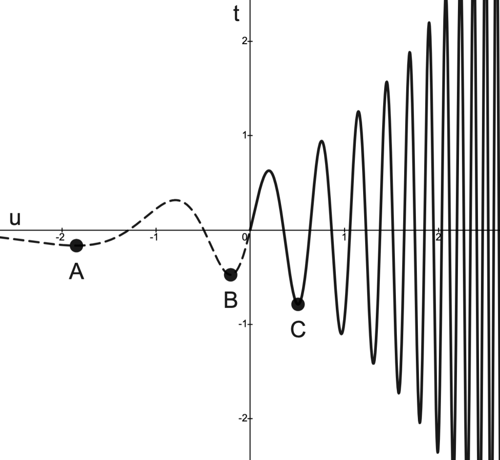
.
.

.
.


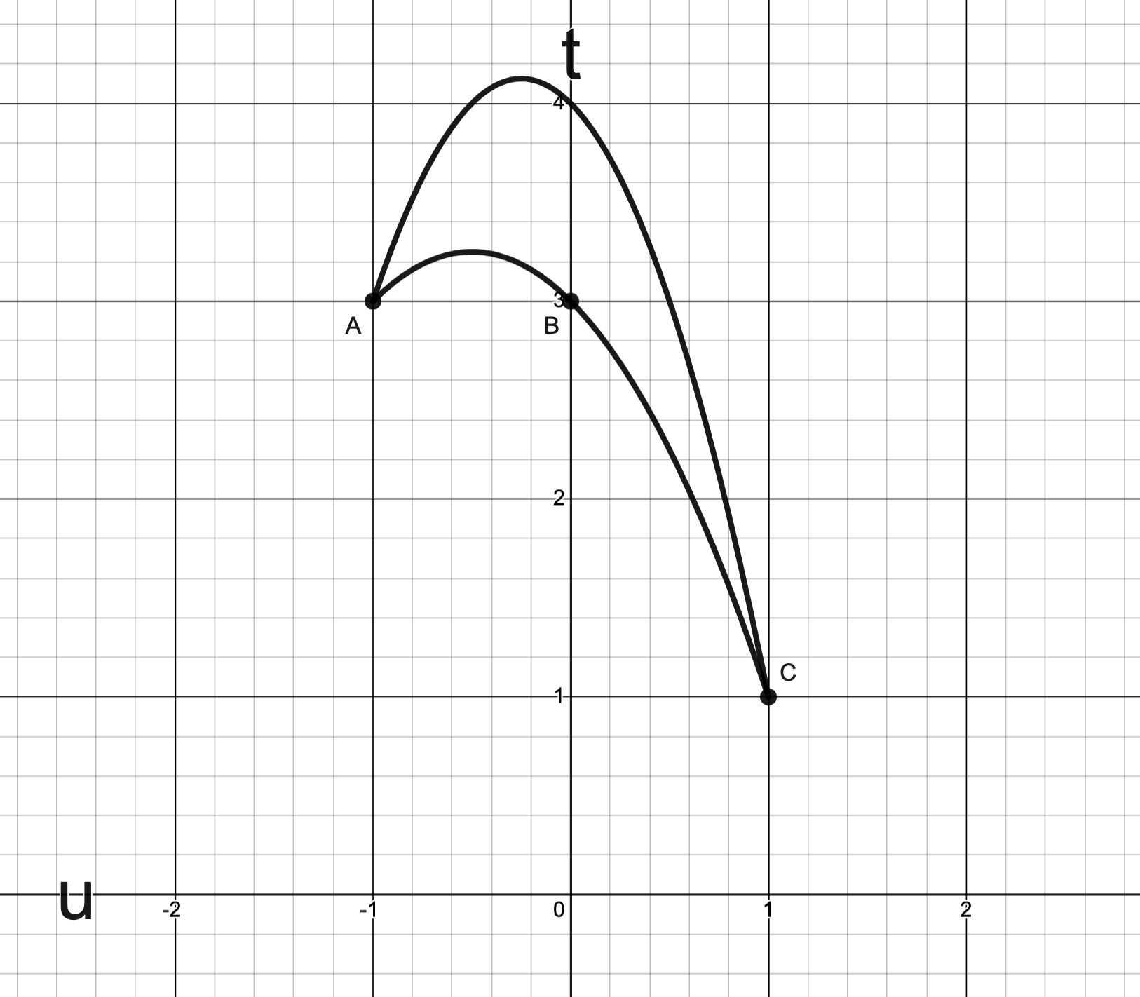
 , define the function

 iff
iff  and
and  for some
 is exactly the Lagrangian


 is finite.)


 , we conclude weak duality:


;
given as the

 :
:

 .
. .
.
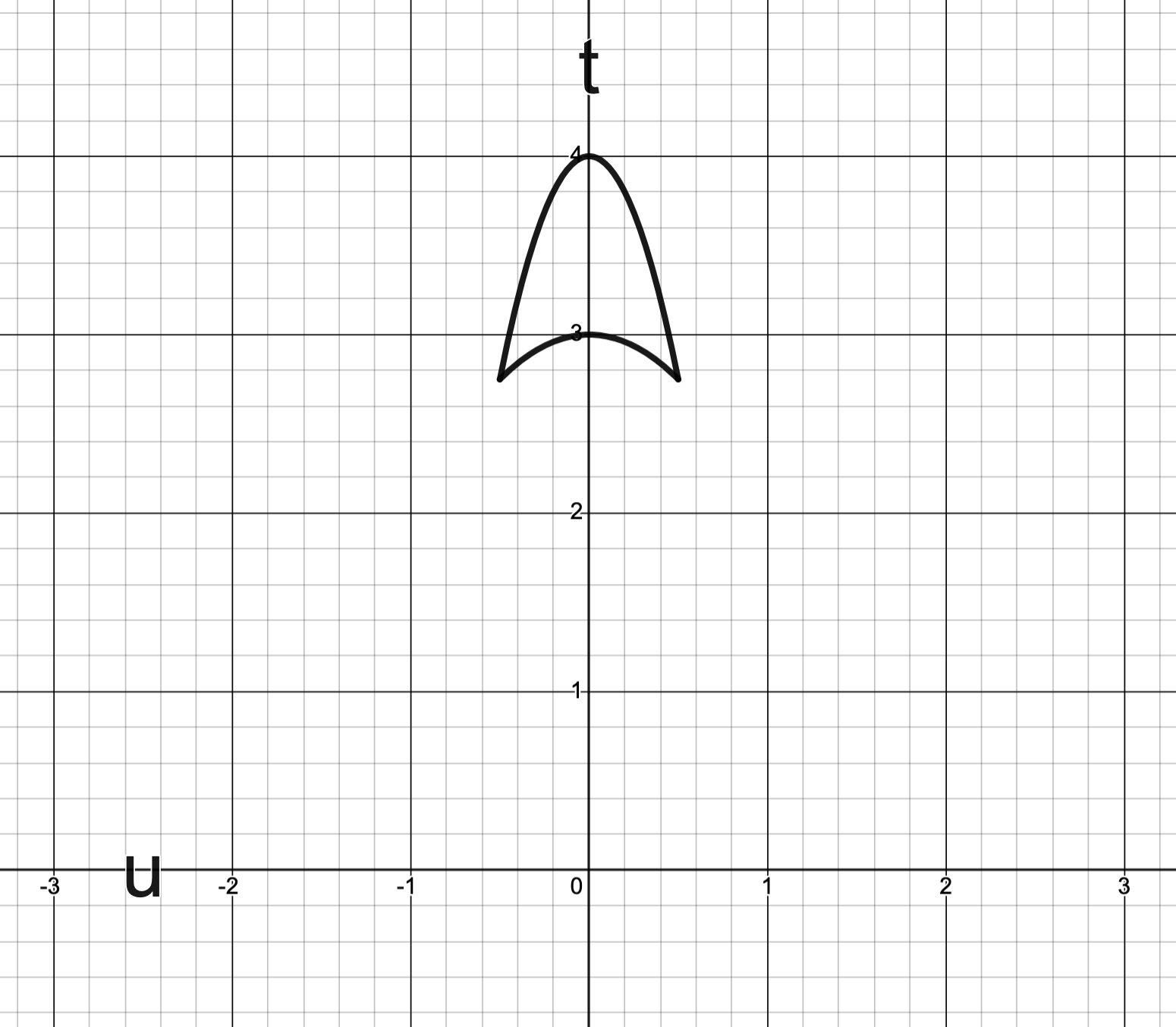

 are convex.

 is in
is in  .
.
 are given.


 convex.
 and
and ![s \in [0,1]](https://s0.wp.com/latex.php?latex=s+%5Cin+%5B0%2C1%5D&bg=ffffff&fg=111111&s=3&c=20201002) , then
, then
gives
gives


 .
.
 of
of  of
of 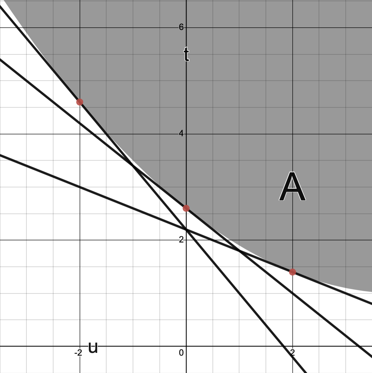

 of
of  .
.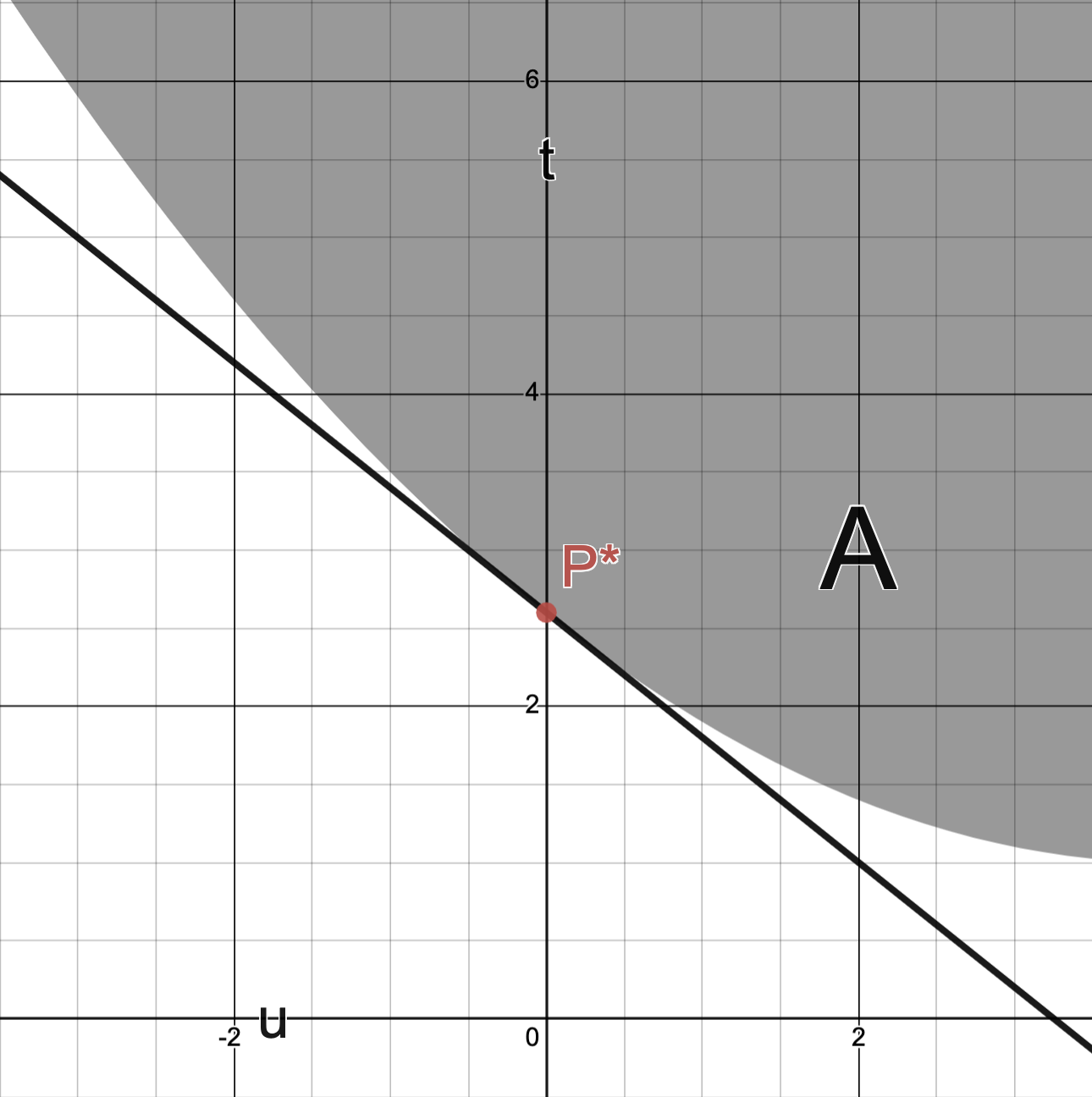
 with
with  .
. be such that
 .
. is to the right of
  .
. and lies above
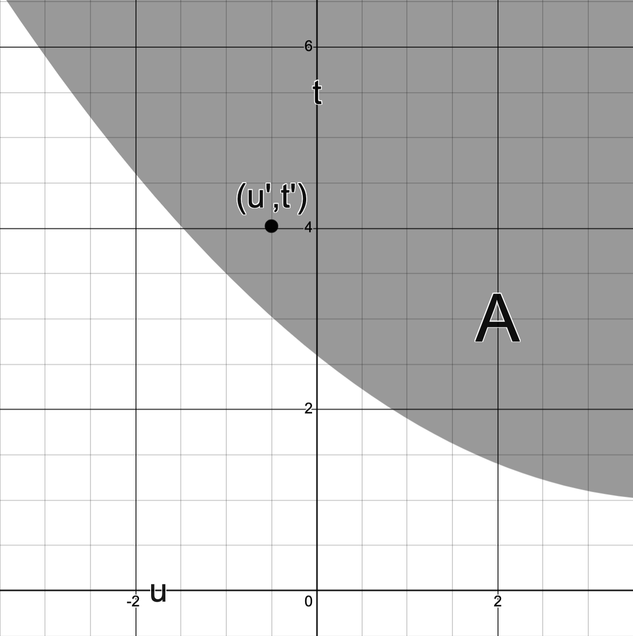
 .
.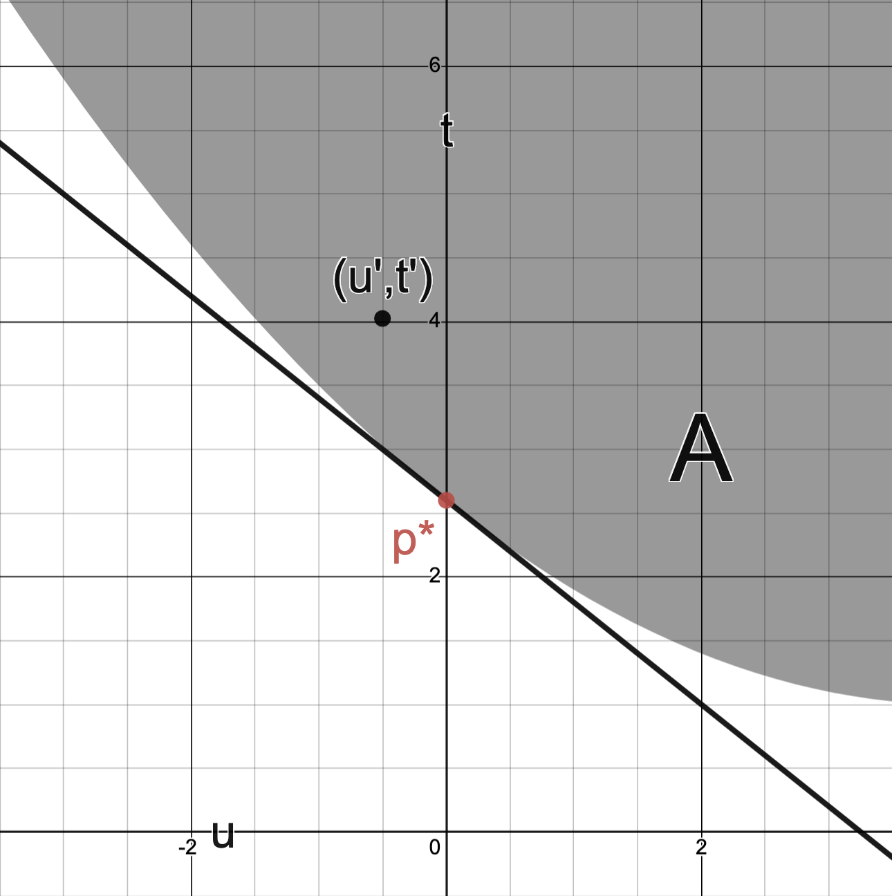

 were the case, then the line
  would fail to be a supporting hyperplane since it will pass through
  .
. may be decreased or is unachievable.
 with
with  is depicted below.
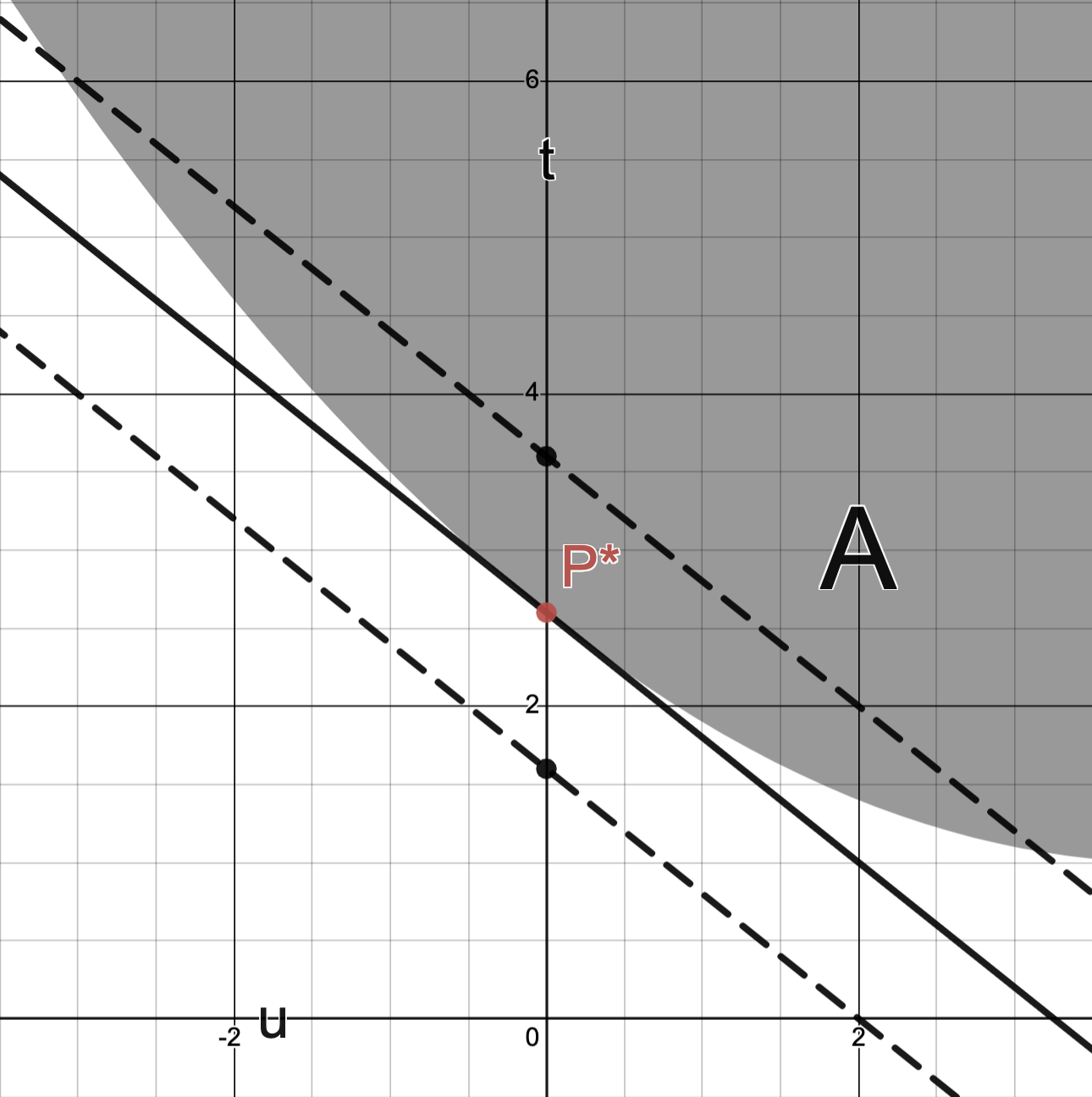


 , the Lagrangian is

 .
.


 :
:

 , we conclude

 with
with  , then

 may be is 0.


 .
.


 satisfy
  .
.
infeasible
.
infeasible
.
.


is continuous.
 .
.


 are step sizes and
  are search directions vector.
 may depend on
  .
. determines how far to step and in what direction from
 , then continuity would give
and terminates search when an iterate
satisfies this tolerance:
needs to be chosen.
depends on the step; if
is independent of the step, then
is called stationary.


 , and a stopping criterion

 .
repeat: compute
.
repeat: compute  .
until:
.
until:  .
.

 , then
  .
.

, we have
.
being closed holds in case
and
.
is an open ball in
 such that

indicates the identity matrix.
and let
with eigenvalue
and
.


 such that

to conclude each of its matrix entries are bounded.
there exists
such that
implies
and
in previous step, there holds
is continuous on a compact set.
for sufficiently large
.


 gave a lower bound on the eigenvalues of
  provides an upper bound on the eigenvalues.
 there holds

.
we have


 satisfies
  -tolerance.

 , which gives


 , we conclude


 are two minimizers, then
  since
since

 such that

 satisfying
is defined via
and
are chosen so that the sequence satisfies descent:
whenever
.


.
or
as short hand for
.


 to satisfy descent, it is necessary that

 to both sides of

 satisfying

 form an acute angle.

 sufficiently small so that

 , a general descent algorithm takes the following form.
 repeat:
1. Determine descent direction
repeat:
1. Determine descent direction  .
2. Choose step size
.
2. Choose step size  .
3. Take step:
.
3. Take step:  .
until: stopping criterion holds.
.
until: stopping criterion holds.

 .
. minimize
  .
. .
. .
3. Take step:
.
3. Take step:  .
until: stopping criterion holds.
.
until: stopping criterion holds.
be sequence of exact step sizes and let
and so the sequence
satisfies descent:
.


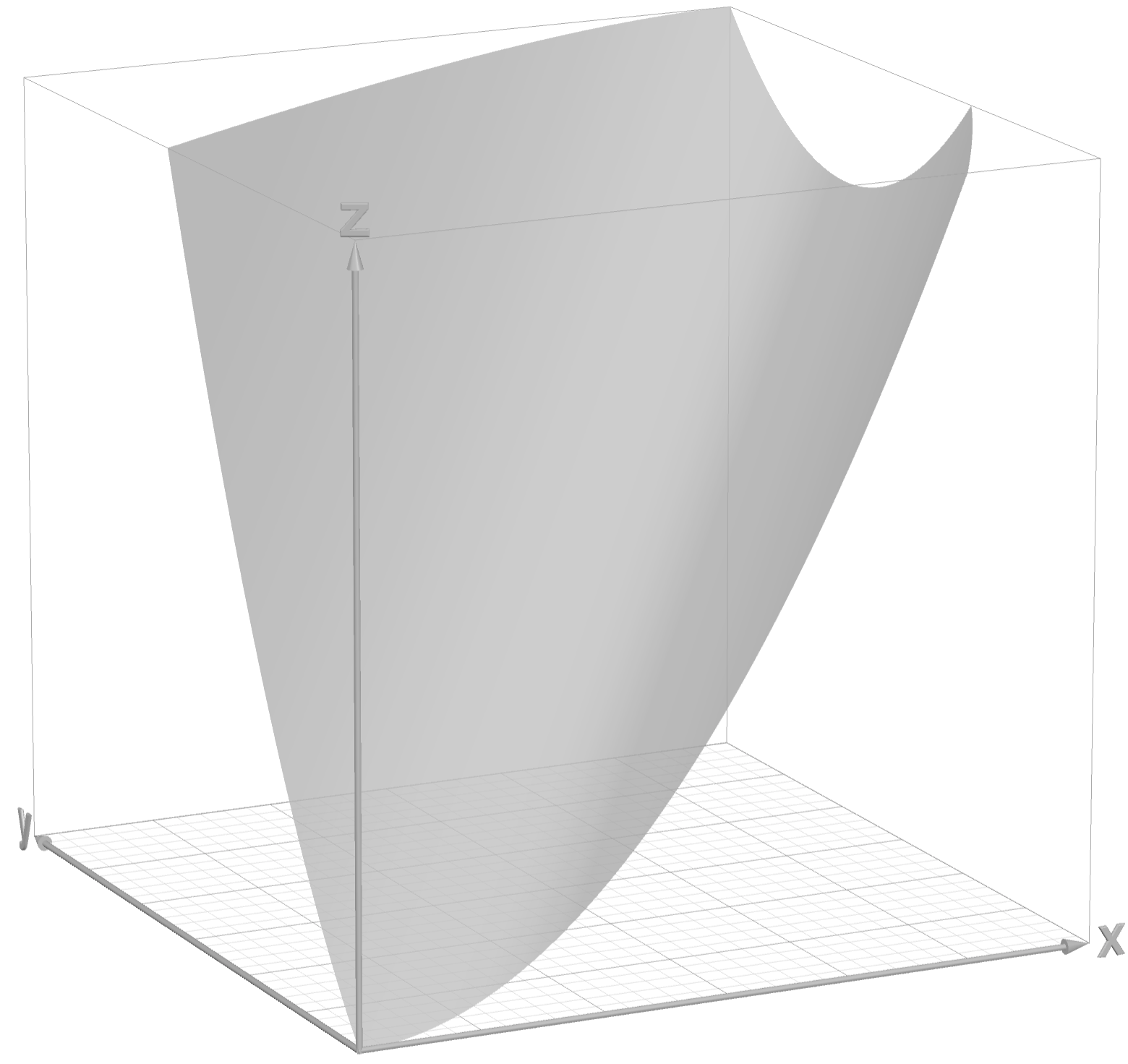

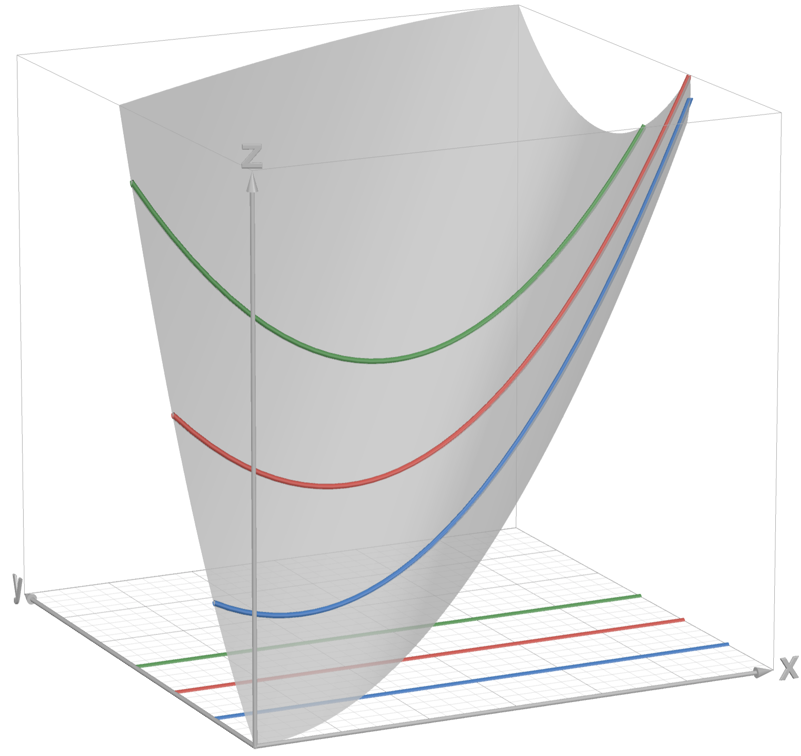
 obtained from exact line search on each respective line.


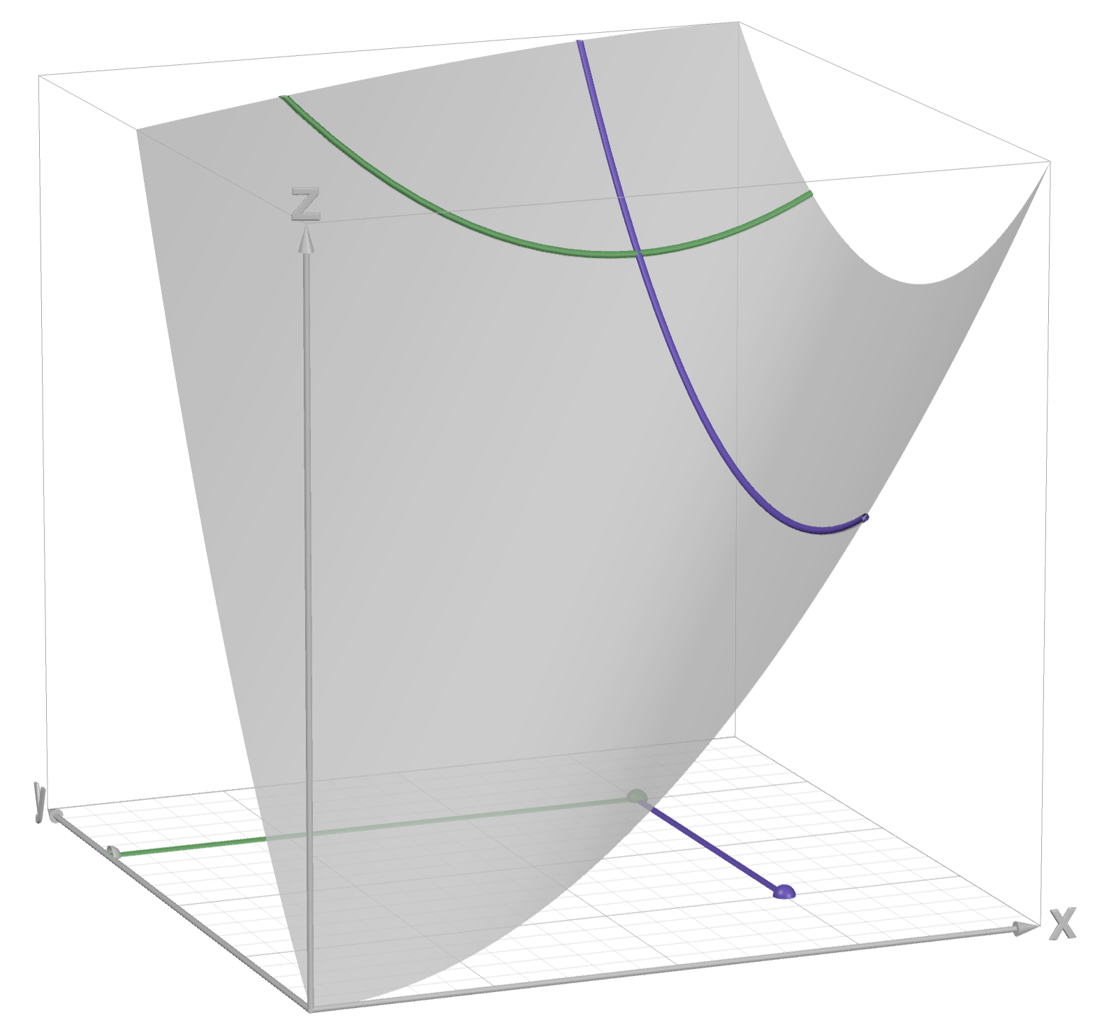


 ,
,
until the decrease


 results in an increase in objective, convexity ensures
  results in decrease for some
  .
.
and
.

.
.
, the difference
is a linear approximation of the difference
.
, the inequality in 3. is guaranteed for small
, then
.
which guarantees a decrease comparable to the decrease predicted by linear extrapolation.


such that


 at
at  parameters
 while:
  update:
.
, it also holds for all
.
such that
and Armijo’s condition are sufficient for convergence of gradient descent coupled with backtracking line search, which is detailed below.
is, the faster
decreases and hence the quicker the Armijo-Goldstein inequality holds.
.
is well-defined to start the algorithm, i.e., that
.
with
.
be in the “small


 .
2. Perform line search to determine step size
.
2. Perform line search to determine step size  .
3. Take step:
.
3. Take step:  such that

is bounded in terms of the problem data:
,
 and its initial sublevel set
  , then


 and
and  such that

 .
.

 for resulting exact line search step size.
 for the next iterate after
 :
:

 with
with  .
.


 using gradient descent and exact line search to find
  .
.
 in place of
  , we conclude


 , conclude
  as
as 
 and so there holds convergence.


 .
.
implies
,
While the RHS is independent of knowing 
 and its initial sublevel set
  .
Lastly, if the desired tolerance is
.
Lastly, if the desired tolerance is 
 be fixed but arbitrary and let
  .
. .
.


 gives
gives


 , we conclude


 .
.,

 .
. .
. and termination happens at
  , which consequently satisfies
  .
. , then


 , then


 , let
, let


.
.


provides a means of measuring relative eccentricity between any two directions; e.g.,
than
.
is independent of the placement of
, let
.


.
.
be convex subsets with
.


 measures a lack of symmetry and indicates
  does not indicate
 ; e.g., Reuleaux triangles are of constant width.
be convex subsets with
.
and
, then
is an ellipsoid and all ellipsoids can be described like this.
.
.
and therefore need to first compute
would imply
, which is a contradiction.
and so complementary slackness implies
gives
gives


 for some
  .
.
 .
. , let
, let

 .
. is controlled by the conditioning of
can be taken to be arbitrarily large and
, the worse (larger)
 .
.
 depends on
  , then
  and so we may take

 .
.
 be as above.
Then
be as above.
Then


 ):
):

 .
.

 is estimated in terms of the extremal widths of
  and
and  .
.
 .
.

 .
. .
.


 .
.


 .
.


 near
near 


 .)
.)

 .
.

 are
are


 .
.
 be the initial point and define the initial sublevel set


 and
and  for an arbitrary
  .
.
 are of the form

 .
. than
than  .
.

 considering the step

 .
.
 , this is unsurprising since the larger
  , then Taylor’s approximation gives


 , we conclude


 so that

 -coordinates is likely to behave well when minimizing
  .
.
 -coordinates is

 :
:


 in the original variables.
 is a function
  satisfying
for all
.
for all
.
satisfies
, then
.
:
norms for
:
norm:


 , the unit norm sphere

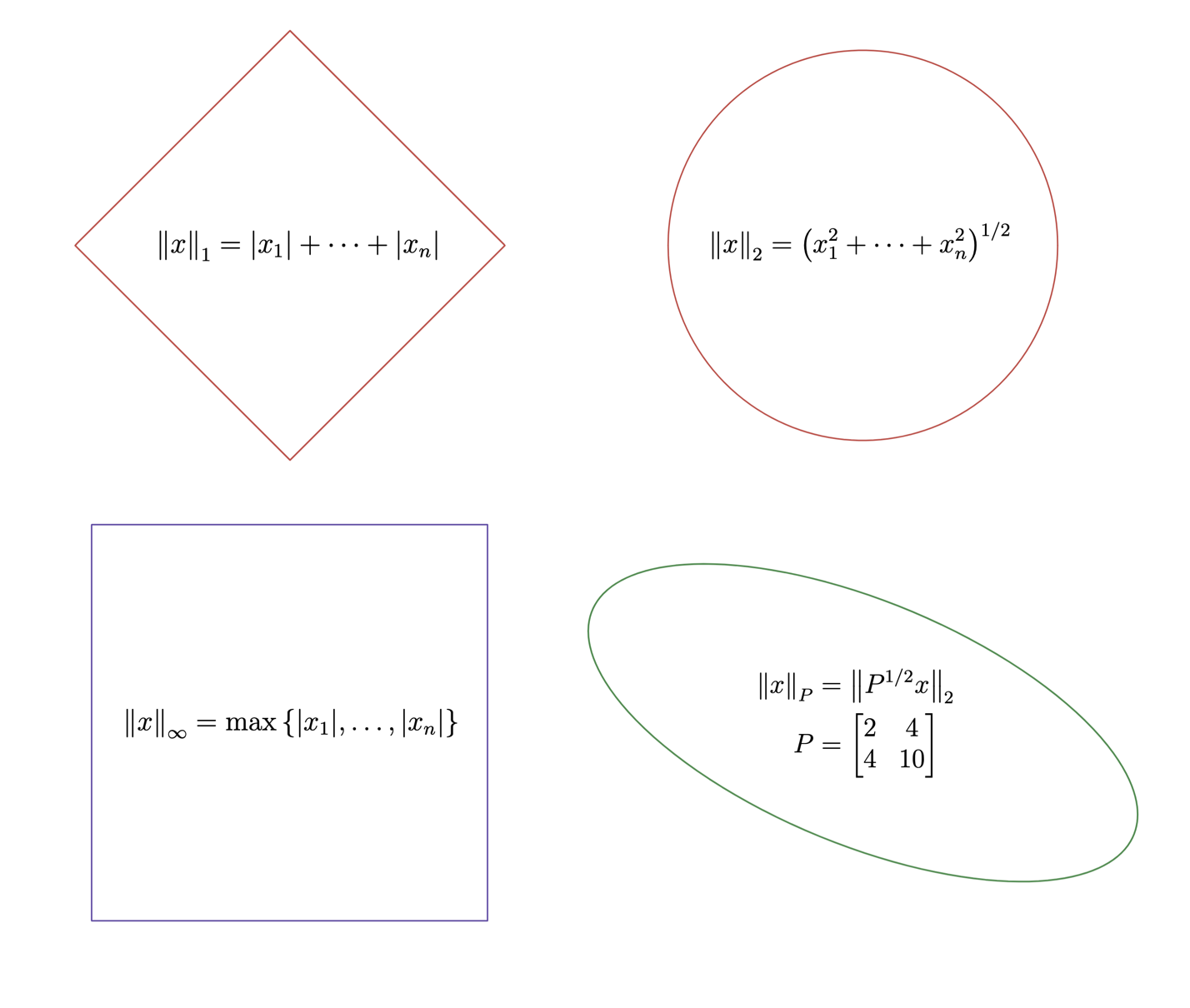
 to be
to be

 .)
.)
 , for
, for 


 , for
, for 
 , where

 (for small
  .
.is generally not unique; e.g. this can occur for
and the black dots indicate two distinct
.
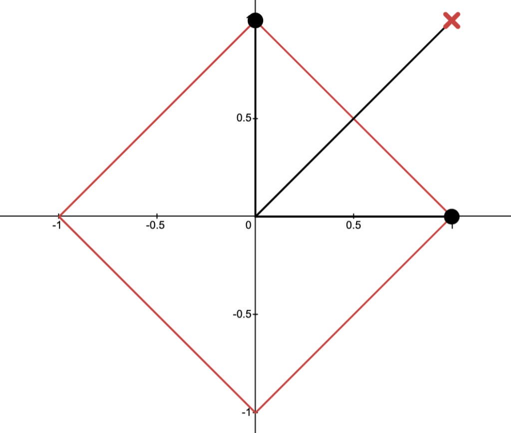
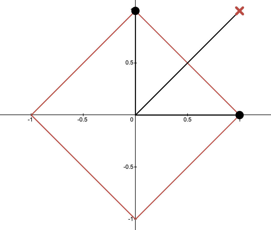


instead of
, we have


 .
2. Perform line search to determine step size
.
2. Perform line search to determine step size  .
until: stopping criterion holds.
.
until: stopping criterion holds.

 .
.


 .
.


 is
is


 and
and

 in the new variables

 is equivalent to standard gradient descent in a different coordinate system.
 may result in a well-conditioned problem in the new variables

 be such that

 denote the standard basis of
  .
.


 , then convexity implies

 is a descent direction.
 .)
.)
 may lead to efficiently solving system.


.
of
.
for
.
part of
.
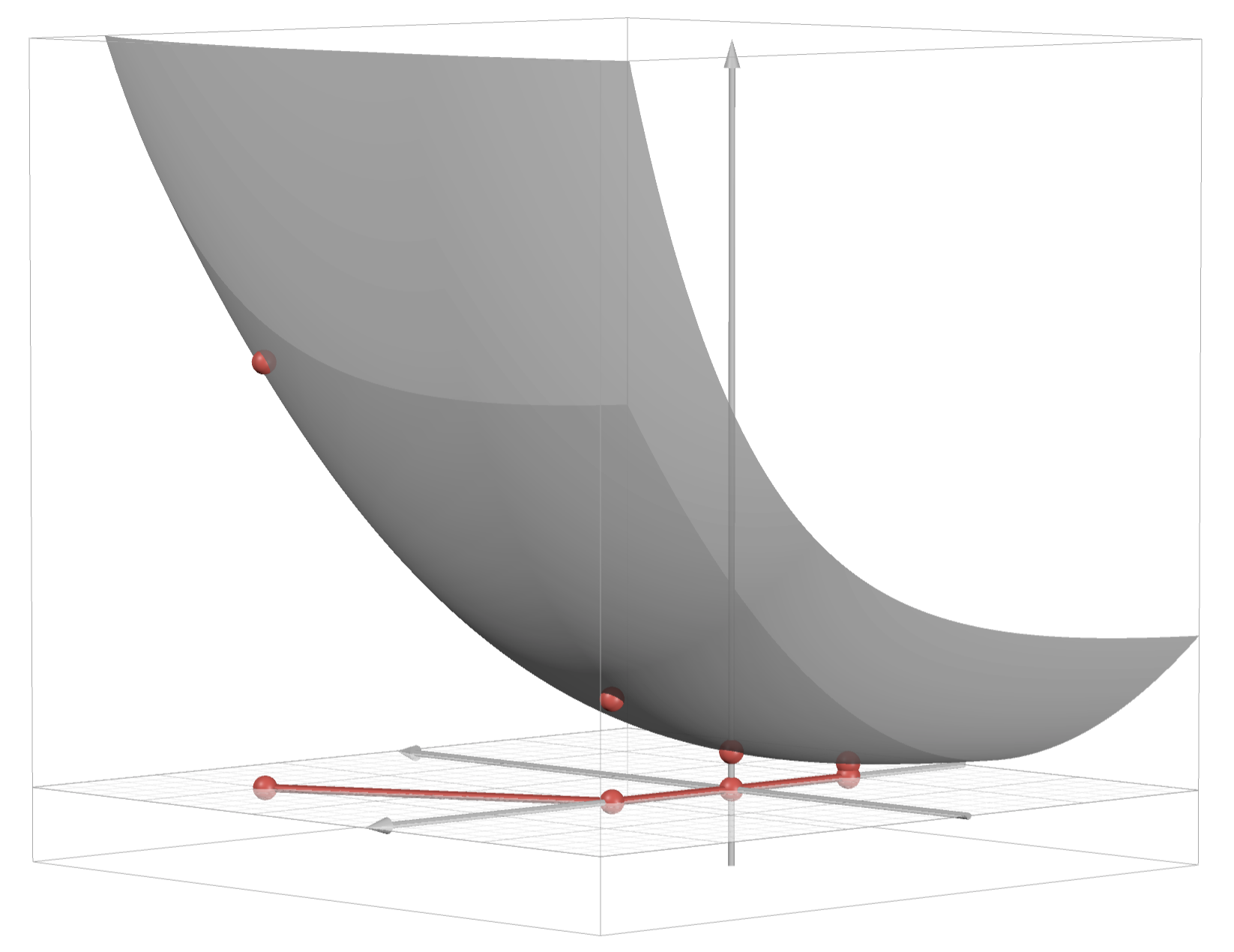


 is
is

 :
:


 is the second order Taylor approximation of
  is a convex quadratic in
 is minimized at

is a good approximation for
.
and
.
This conclusion is depicted below.
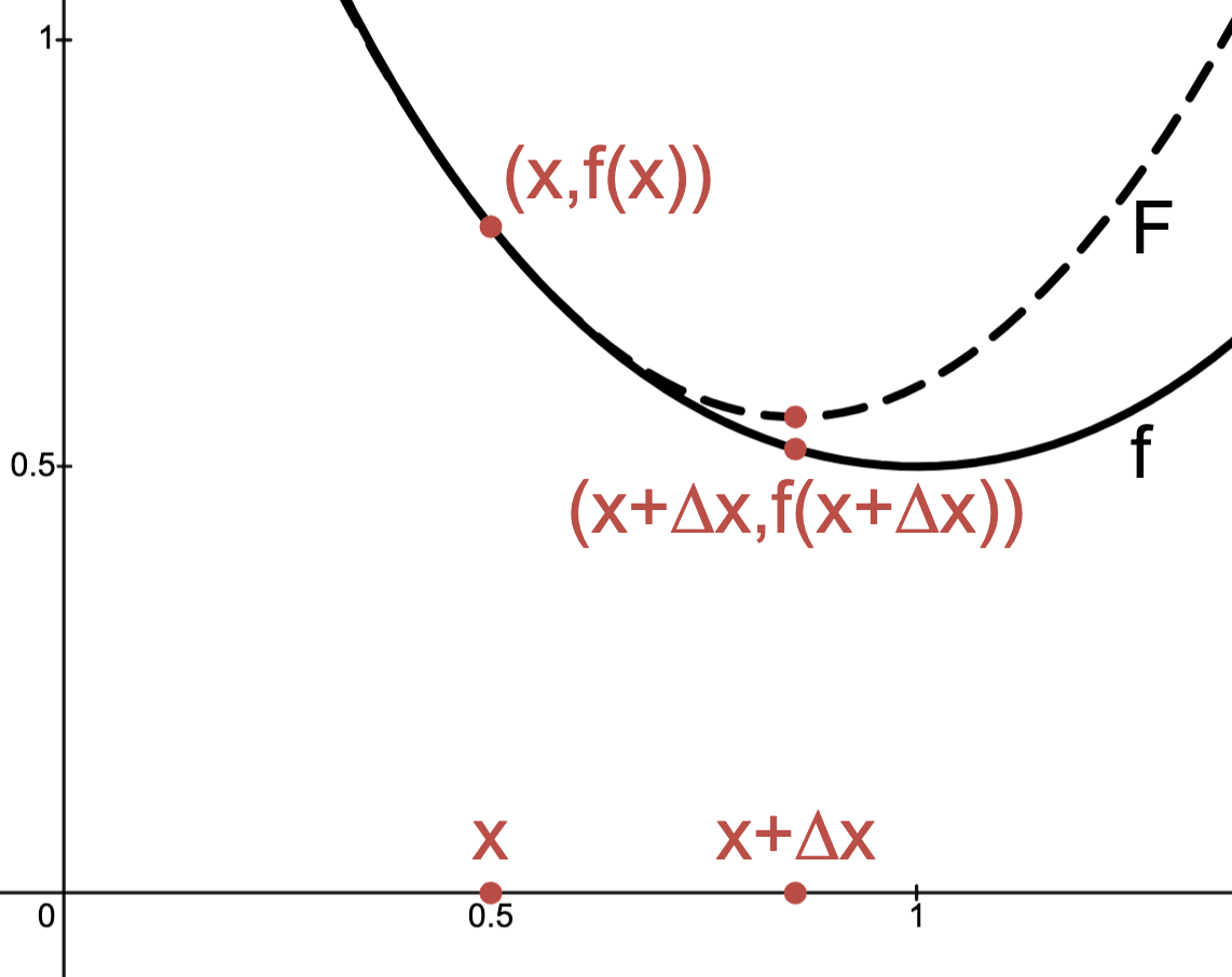

 is used to estimate


 .
.


 and
and
 .
2. Stopping criterion: quit if
.
2. Stopping criterion: quit if  .
3. Perform line search to determine step size
.
3. Perform line search to determine step size  .
.
is nonsingular


 for
for  for
for 


 via Newton’s method with
  gives
gives  .
.
 .
.


exists.
with
.
indicates equality constraints are independent (not superfluous).
indicates there are fewer equality constraints than variables.
 .
. remains feasible?
.

 .
.
 such that

 .
.


 solves

 solves

 to solve original equality constrained problem.


 is not a priori twice continuously differentiable, even if
  is twice continuously differentiable, then can use unconstrained optimization to find dual optimizer


 as above.


 with
with  :
:

 solves

 approximates
  is so that
 .
. is feasible for all
 .
.

, and


 gives a suitable stopping criterion as before.
 is feasible.
 tolerance
  repeat:
1. Solve
repeat:
1. Solve
 .
2. Stopping criterion: quit if
.
2. Stopping criterion: quit if 
is continuous.
exists.
that is primal feasible, then primal optimal is
.
having unique solution.
to be optimal.


 is the dual optimal value and strong duality holds, then


 .
.


 recovers unconstrained Newton step.


 (solid curves) and
  (dashed curve) are plotted below.
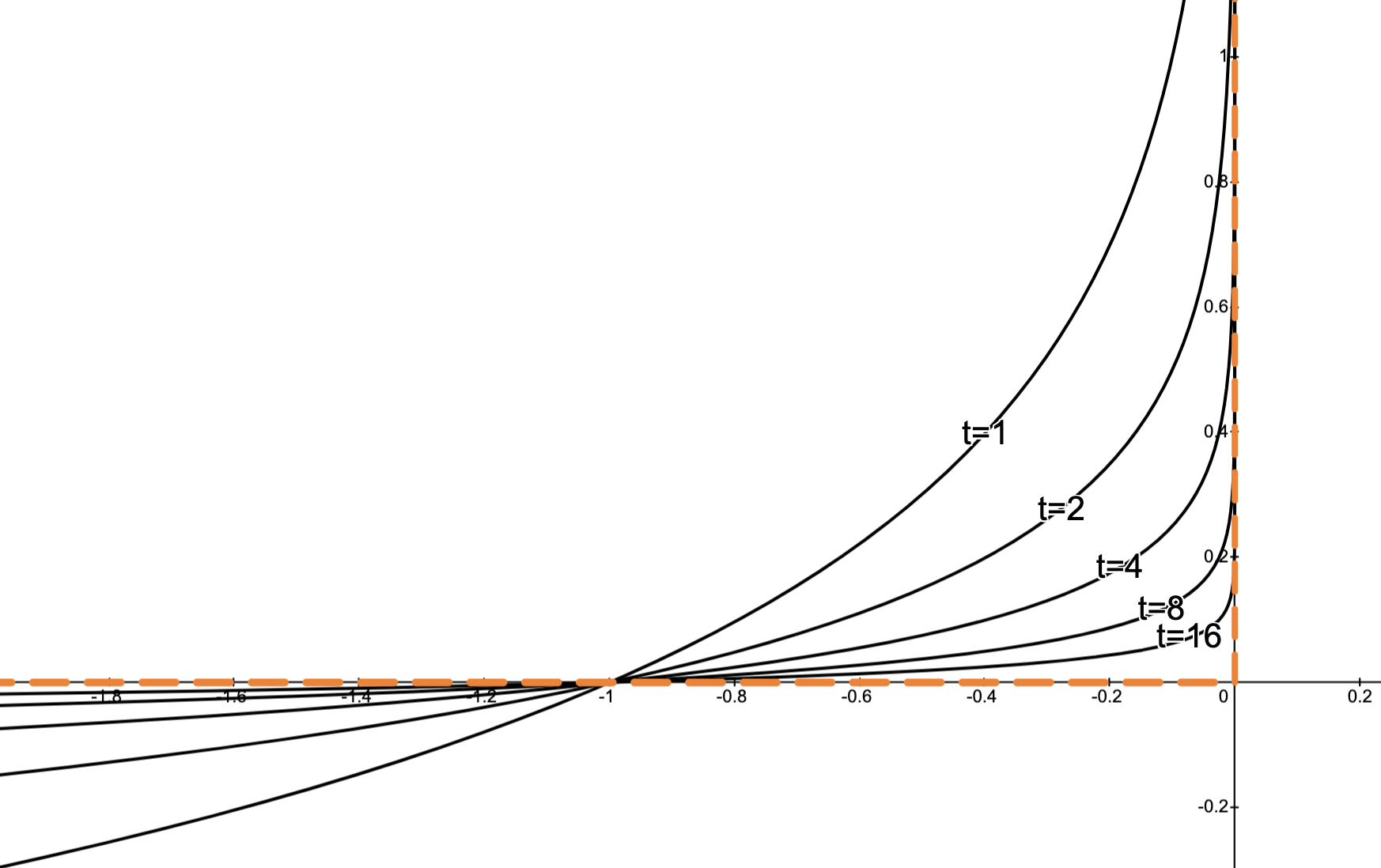

 , we have

 and fixed
 approximates
  well for large


for
and so
penalizes
controls this penalty since
.
are twice continuously differentiable, then so is
on its domain
convex implies
is convex, and so
is also convex.
, and prove
as
.
.
:
is an
matrix.


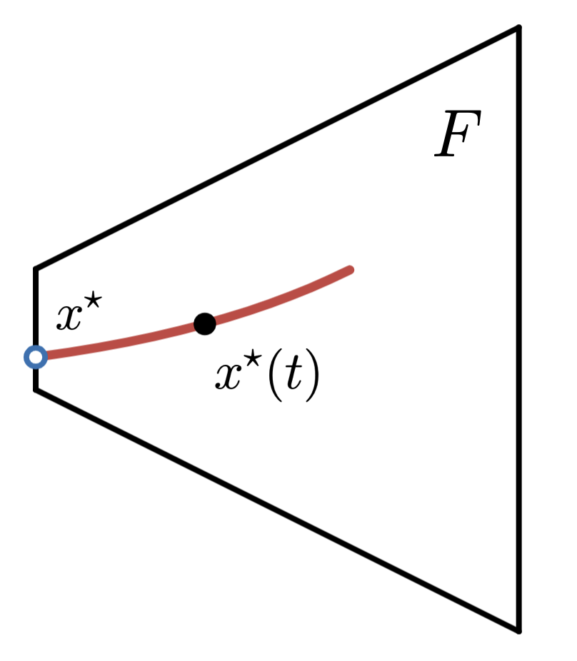

 .
. .
.
naturally determines a path of dual feasible points
.
as
.
 .
.


.
.
paired with the optimality gap gives:


 is convex and so, since

 initial time
  multiplier
  tolerance
  by solving
 with initial point
  .
3. Stopping criterion. quit if
.
3. Stopping criterion. quit if  .
4. Increase
.
4. Increase  .
.  .
.
dictates trade-off between number of inner and outer iterations:
small:
.
.
and
, where algorithm requires one outer iteration.)


 the Newton step for solving the nonlinear system
  .
. solves
  near
near  .
.


 solves this system, then


:
measures divergence from
measures divergence from
measures divergence from
means


 satisfying
  results in a Newton step


 need not form a sequence
  of feasible points.
 need not measure the duality gap.
 satisfying


 is duality gap.
 can be used to define stopping criterion.
 and
and  small
small  nearly duality gap.
 initial
  and
and  multiplier
  repeat:
1. Determine
repeat:
1. Determine  2. Compute primal-dual search direction
  3. Perform line search and update.
Determine step length
3. Perform line search and update.
Determine step length  and set
  .
until:
.
until:  ,
,  and
and  .
.
corresponds to a duality gap of
.


 , we find


 , we find


