These are notes used for lecturing ECSE 507 during the Winter 2024 semester.
Please note that these notes constantly evolve and beware of typos/errors.
These notes are heavily influenced by Boyd and Vandenberghe’s text Convex Optimization.
I appreciate being informed about typos/errors in these notes.
Click each subject to unfold.
Introduction
General Problem
Interested in solving and studying minimization problems subject to constraints:

-
are problem parameters;
-
is the objective function and
usually interpreted as cost for choosing
;
-
is a constraint set often described “geometrically”.
Example 1. Design Problem Interpretation
Let=scalar-valued design variables
(e.g., dimensions of manufactured object, yaw and pitch of jet).= penalty for choosing design
(e.g., cost in material, energy, time, deviation from desired path).= design specifications
(i.e., allowable/possible values for).
E.g.,specifies minimum and maximum design values.
which minimize cost  and satisfy the design specifications
  .
.Example 2. Minimize function over ellipse
Let-
-
.


It has two solutions:
 .
.Many applied problems can look like this, but with an applied interpretation.
Problems With Structure
General optimization problems can be numerically inefficient to solve or analytically difficult, unless and have additional structure/properties.Identifying nice structure/properties of problem
 problem may become analytically solvable or numerically efficient.
Examples of nice structure:

 defined in terms of linear equalities/inequalities;
e.g.,
 , or succinctly written
  .
.
E.g., convex if

 is itself a convex set.

E.g.,
 and given by
If
 sparse
 lots of cancellation improve computational efficiency

Linear Programming
Simplest case: is linear and defined in terms of linear constraints.Notation: if
 , then


 = transpose of the column vector
  .
.Linear program: given
,  ,
,  , solve

 and
and  .
.
Positives of linear programming:
- Conceptually simple: relies heavily on linear algebra
- There are classical numerical methods which are often very efficient.
- If
is local minimizer of
- Can sometimes approximate smooth problems linearly; however, usually can only give “local” results.
(E.g.,for
.)
Shortcomings of linear programming:
- Many applied problems are not linear.
- Many problems may not even be (suitably) approximated by linear programs.
E.g., the “barrier”
is better approximated by the a “logarithmic barrier” of the formthan any linear function.

Convex Optimization
Convex optimization problem: and are convex.This is the main focus of the course.
Positives of Convex Optimization:
- Relatively conceptually simple.
- Still often have efficient, albeit more sophisticated, numerical methods.
- Many applied problems may be recast as or approximated by convex optimization problems.
- If
Shortcomings of Convex Optimization:
Example (Least Squares)
A standard and ubiquitous kind of convex optimization problem is the least squares problem.This problem takes the form:

is some norm
is the (convex) objective function
are convex.
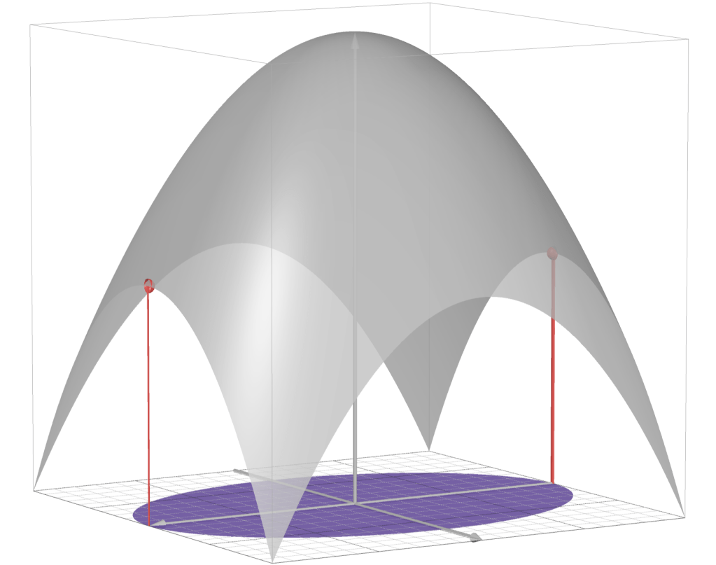
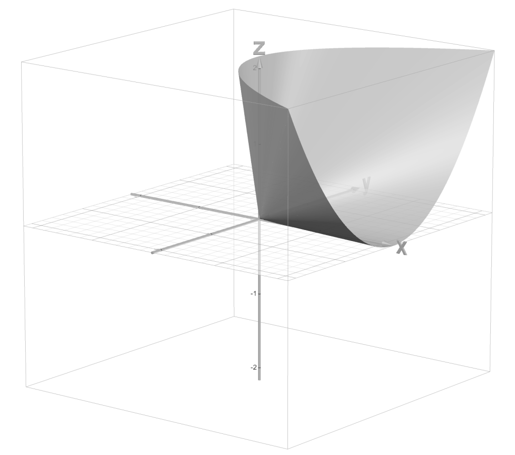
Example: Distance from points to ellipse
If ,
,  is the identity matrix, and is an ellipsoid, then the solution is the point in the ellipsoid closest to the point
  .
.The image below depicts this situation with


 .
.
Optimal Control
Let-
be functions
.
 evolves by

-
is the time derivative of
-
are assumed to be given;
-
we think of
;
- we think of
as an input we are allowed to choose to dictate the evolution
; i.e.,
- When
, the system experiences “feedback.”
-
the goal: choose control law
so that
Example: Optimal Control Problems
Optimal control problem: choose the “best” control which gives the “most” desirable .
Typically “best” and “desirable” are determined by size/cost of
and ; e.g., one may wish to minimize


Rough Outline of Course
- Part 1: Basics of Convexity and Convex Optimization Problems.
- Part 2: Applications of Convex Optimization Problems.
- Part 3: Algorithms for Solving Convex Optimization Problems.
- Part 4: Topics in Optimal Control.
Convex Geometry
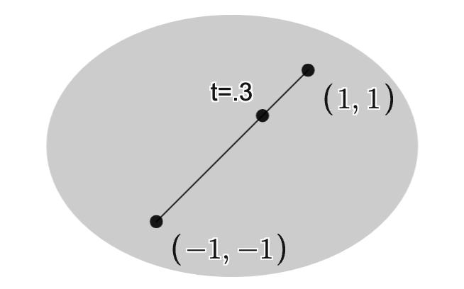
Convex Sets
Convex set: a subset satisfying:
for all 
![t \in [0,1]](https://s0.wp.com/latex.php?latex=t+%5Cin+%5B0%2C1%5D&bg=ffffff&fg=111111&s=3&c=20201002)

 contains all line segments whose endpoints belong to .
Examples: some standard convex sets.
- Closed or open polytopes in
.
E.g., the interior of a tetrahedron. - Euclidean balls, ellipsoids.
- Linear subspaces and affine spaces (e.g., lines, planes).
- Given a norm
with centerand radius
is a convex set.
Recall: a norm satisfies-
for all vectors
;
-
for all vectors
;
-
iff
.
-

Affine Subsets
Affine subset: A subset satisfying:
For all 
contains all lines which pass through two distinct points in .N.B.: An affine subset is just a translated linear subspace:
“a linear space that’s forgotten its origin”.
Example 1.
Let be the
  -plane in
  .
. Then any translation or rotation of
is an affine subset.
Example 2.
If, , then  is affine.
 (
is just a translate of  .)
.)
Example 3.
Let

 is
is

 translated by 3 in the
  -direction:

Cones
Cone: A subset satisfying:
For all 


contains all “positive” rays emanating from the origin and passing through any of its points.Proposition.
is a convex cone iff for all  and
and  , there holds
  .
.
Proof.
Step 1. ()
Suppose is a convex cone and let and be arbitrary.Want to show:
 .
.
Step 2.
Being conic implies and
and  belong to for all
  .
.
Step 3.
Being convex implies , as desired.
Step 4. ( )
)
Suppose is such that for all and .Want to show:
 is a convex cone.
Step 5.
being conic follows from taking  arbitrary and
  .
.
Step 6.
Convexity follows from taking with
with  and
and  .
.Indeed:
 and
and 
 for
for  since
since  .
.
Examples.
- Hyperplanes
with normal
,
halfspaces,
nonnegative orthantsare all convex cones.
(Here,if
for
.)
-
Given a norm
on
which is a convex cone in,
.
- See “positive semidefinite cone” below.
Polyhedra
Polyhedron: Any subset of the form


 and scalars
  .
.
Thus,
is a finite intersection of halfspaces and hyperplanes.N.B.: Introducing equality constraints can be used to reduce dimension.
Example.
The polyhedron below is given by the indicated system of inequalities:


 for suitable
  .
.
Positive Semidefiniteness
Symmetric matrix:
a matrix satisfying
  ; i.e.,


Positive semidefinite matrix:
 satisfying
  for all
  .
.Equivalently,
only has nonnegative eigenvalues.
If
is positive semidefinite, then write  .
.If
 and
and  , then write
  .
.Set of symmetric positive semidefinite matrices:

 is not the same as component-wise inequality, as was the case for vectors.)
Positive definite matrix:
 satisfying
  if and only if
  .
.Equivalently,
only has positive eigenvalues.If
 is positive definite, then write
  .
.If
 and
and  , then write
  .
.Set of symmetric positive definite matrices:

Example 1
Let .
.Since
 has positive eigenvalues
  , it follows that
  .
.To see
explicitly, observe

with
 iff
iff  .
.
Example 2.
Let .
.Since
 has nonnegative eigenvalues
  , it follows that
  .
.To see
explicitly, observe

 for
for  and so
  .
.
Example 3.
Let .
.One can conclude
 by showing that
  has positive eigenvalues
  .
.To see it directly, compute

 ) of this quadratic satisfies
  , from which we conclude the polynomial is positive unless
  and hence
  .
.
Example 4.
Let .
. We can conclude
 , either compute its eigenvalues
  or observe that
  and whence
  cannot have only nonnegative eigenvalues.
Positive Semidefinite Cone
Proposition 1. is a
is a  -dimensional real vector space and
  is a convex cone in .
Proof.
Step 1.
is a vector space:
if  and
and  , then it is easy to see:

 .
.
Step 2.
 :
:
since  implies
  , we have the identification

indicate the unique contributions to making  .
.Counting the number of bold entries shows
has entries and hence  .
.
Step 3.
is a convex cone:
For ,  and
and  there holds

 .
.By the proposition in Convex Geometry.Cones, we conclude the desired result.
Proposition 2.
 iff
iff


Proof.
Step 1.
Let

recalling that
 iff
iff  for all
  .
.
Step 2. (Case  )
)
First compute


):  iff
iff  .
.Can thus conclude (in case
):


Step 3. (Case  )
)
Completing the square gives


iff


, take  .)
.)
N.B.: strictly speaking,
 was not used anywhere; however,
  immediately implies
  , and
, and  also implies .
Step 4.
Putting Steps 2. and 3. together, we conclude: iff
Image of 
In light of Proposition 1 and Proposition 2, we can plot


Separating Hyperplanes
Let be two sets.
Separating hyperplane: a hyperplane given by

 and
and  such that

 is said to separate and .
Thus,
cuts  into two halfspaces with one containing all of and the other containing all of .
Separating Hyperplane Theorem. If
are two disjoint convex sets, then there exists and such that is a separating hyperplane which separates and .
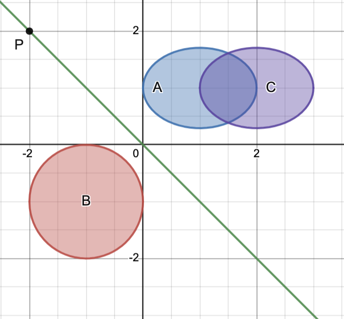
Example 1.
Consider the convex sets

Note that
 separates the pairs
 ![[B,A]](https://s0.wp.com/latex.php?latex=%5BB%2CA%5D+&bg=ffffff&fg=111111&s=3&c=20201002) and
and ![[B,C]](https://s0.wp.com/latex.php?latex=%5BB%2CC%5D+&bg=ffffff&fg=111111&s=3&c=20201002) .
Moreover, the pair
.
Moreover, the pair ![[A,C]](https://s0.wp.com/latex.php?latex=%5BA%2CC%5D+&bg=ffffff&fg=111111&s=3&c=20201002) cannot be separated since and have significant overlap.
cannot be separated since and have significant overlap.
Example 2.
Consider the convex sets

First note
 since neither contain their boundaries.
As such, they have a separating hyperplane which is given by
.

 with their respective closures
  , the plane still separates .
Indeed,
 for
for  and
and  for
for  .
.
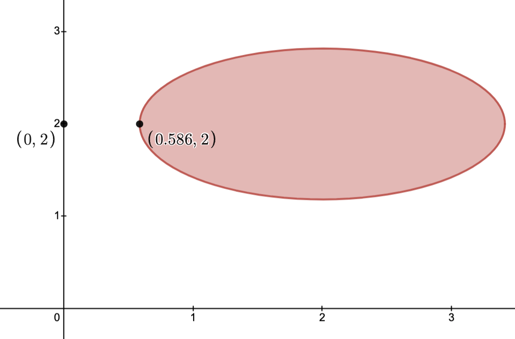
Supporting Hyperplanes
Let be a fixed set and fix a boundary point


and the singleton  , then
  is called the supporting hyperplane of at
  .
.Equivalently,
lies entirely in a halfspace with boundary given by .
(Here:
 indicates the closure of and
  indicates its interior.)
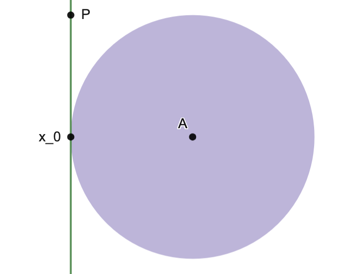
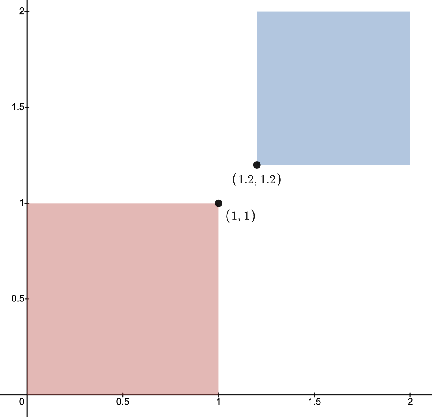
Example.
Consider the convex sets

 .
.
Letting
 , we note
  .
.Next, observing that, if
, then  and so

separates and  , showing that is a supporting hyperplane of at the boundary point ; see image below.
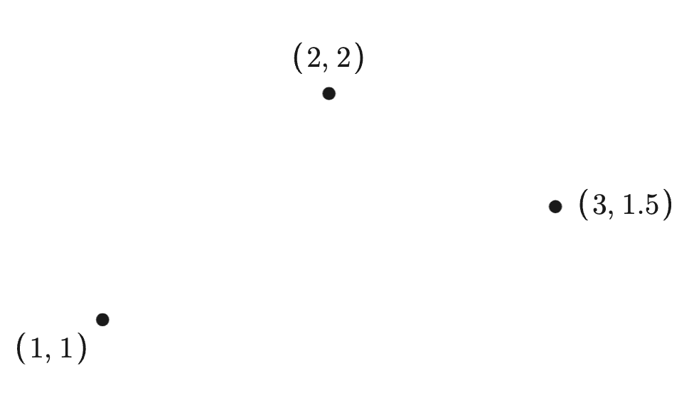
Hulls
Let be a fixed subset. Convex hull:
the set

and is itself convex.
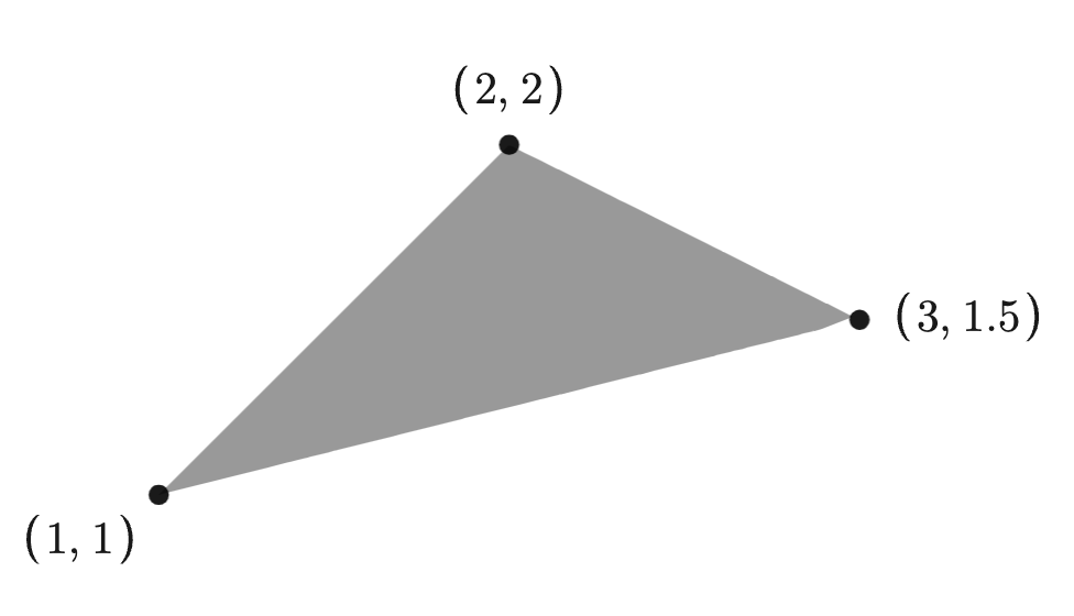
Example: The images below depict a set of three points and its convex hull.
Affine hull:
the set

and is itself affine.
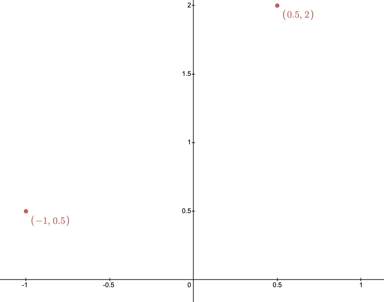
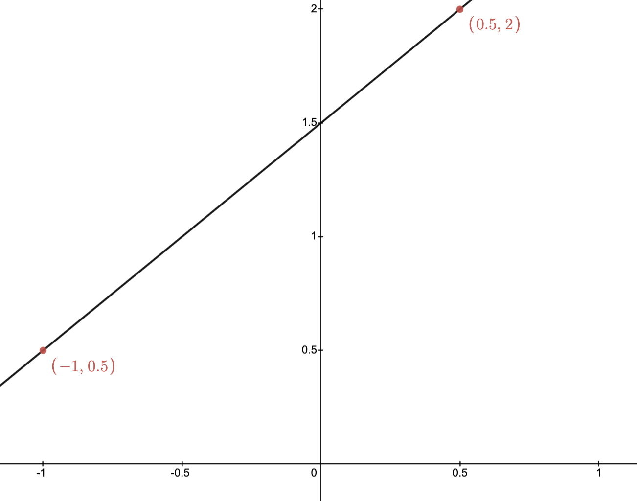
Example: The images below depict two points and their affine hull.
Conic hull:
The set

and is itself a cone.
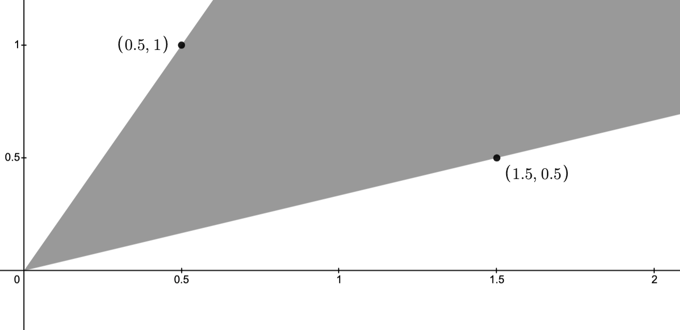
Example: The images below depict two points
 ,
,  and their conic hull.

Details
To see that the conic hull really is the shaded region, note that, by taking and
and  , where
 ![t \in [0,1]](https://s0.wp.com/latex.php?latex=t+%5Cin+%5B0%2C1%5D+&bg=ffffff&fg=111111&s=3&c=20201002) and
and  , the conic hull contains all points of the form
  .
.
Thus, it contains all line segments connecting any two points on the nonnegative rays
 and
and  .
.
N.B.:
- Conic hulls are convex cones.
-
Taking the “___ hull” of
-
The “___ hull” is a construction of the smallest “___” subset containing
Generalized Inequalities
Proper cone: a convex cone satisfying
-
is closed (i.e.,
-
-
.
, a partial ordering  on defined by

 is a partial ordering and so
  is not well-defined for all .
Generalized strict inequality: given a proper cone , a partial ordering on defined by
is not well-defined for all .
Generalized strict inequality: given a proper cone , a partial ordering on defined by

Examples
-
(CO Example 2.14)
If, then
N.B.:.
is the standard inequality on
.
-
(CO Example 2.15)
If, then
.
-
Let
Then.
In the image below:-
.
-
The cone with vertex
depicts those
with
-
The cone with vertex
depicts those
, and so
, as indicated in the image.
Moreover,and
are not comparable.
-

Convex Function Theory
Conventions and Notations
-
Writing
always means a partial function with domain
possibly smaller than
“Function” will mean “partial function.” - If
, we may work with the extension
given by
It is common to implicitly assumehas been extended and to write
and its extension
.
-
Given a set
, its indicator function is
- We write


Convex Functions
Let be a function with convex domain  .
.
Convexity:
for all![x,y \in \text{dom}\, f, t \in [0,1]](https://s0.wp.com/latex.php?latex=x%2Cy+%5Cin+%5Ctext%7Bdom%7D%5C%2C+f%2C+t+%5Cin+%5B0%2C1%5D&bg=ffffff&fg=111111&s=3&c=20201002) there holds
there holds

Strict convexity:
for all there holds

Example: failure of strict convexity
In the figure, the solid line indicates part of the graph of and the dashed line indicates part of the graph of a linear function.
This function fails to be everywhere strictly convex due to linear functions satisfying

Concavity and strict concavity:
when is, respectively, convex and strictly convex.
Remarks.
- It is instructive to compare convexity/concavity with linearity and view the former as weak versions of linearity.
- It is common to extend the definition of convexity to extended functions, i.e., those of the form
.
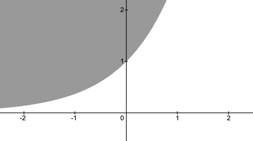
For example, the indicator functionis convex in this sense.
To give insight, consider the image below, where the thick line is the “graph” ofto
for any
.


Examples
- All linear functions are convex and concave on their domains.
-
is convex on
.
-
is convex on
.
-
is convex on
for
or
and concave for
.
-
is convex on
- If
is convex (in the extended value sense).

One Dimensional Characterization
Proposition. Let have convex domain and, given


 by
by


is convex iff  is convex for all
  and such that is well-defined.
Proof.
Step 1.
First note that is convex: it is the intersection of
  with the line passing through
  with direction
  .
.
Step 2. ()
Suppose is convex and let  and be arbitrary.
Then, for
![\theta \in [0,1]](https://s0.wp.com/latex.php?latex=%5Ctheta+%5Cin+%5B0%2C1%5D+&bg=ffffff&fg=111111&s=3&c=20201002) and
and  , there holds

is convex.
Step 3. ()
Suppose now that each is convex.Fix
 and let .
We want to show

 and
and

 .
.Since
is convex, we conclude

is convex.
First Order Characterization
Proposition. If is differentiable with convex domain , then is convex iff

Proof (sketch).
We prove it in case ; the higher dimensional case follows by using that with convex domain is convex iff it is convex as a single variable function when restricted to lines intersecting .
Throughout, let
and .
Step 1. ()
If is convex, then we obtain the following inequalities

Step 2. ()
Supposing

 and add the two inequalities


Remarks.
-
For fixed
is affine whose graph is a hyperplane passing through the point.
Therefore, the inequalitymeans this hyperplane is a tangent plane at
In fact, this plane is a supporting hyperplane of the epigraph
at the point -
The affine mapping
is just the first order Taylor approximation of
Thus, differential convex functions are such that their first order Taylor approximations serve as a global underestimators of


Example.
In the image below:-
solid line is the graph of
;
-
shaded region is the convex set given by
;
-
dashed line is the supporting hyperplane at
given by the graph of
.
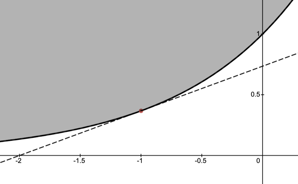
 gives a supporting hyperplane
Second Order Characterization
Proposition. If is twice-differentiable with convex, then is convex iff

Recall: if
 is twice-differentiable, then its Hessian is

Proof (sketch).
Step 0.
The proof is a little more involved, so let us just give two intuitive justifications.Justification 1.
The second order Taylor approximation gives


The first order approximation from Convex Function Theory.First Order Characterization then implies convexity.
Justification 2.
Another intuitive justification is that means the graph of curves everywhere upward like a paraboloid, which evidently suggests convexity.
Remarks.
-
Recall: for
-
for all
Converse is false since

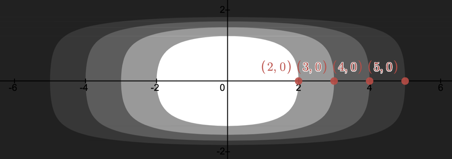
Level Sets
Fix a function and let
 -Level set:
the set

 with
with 
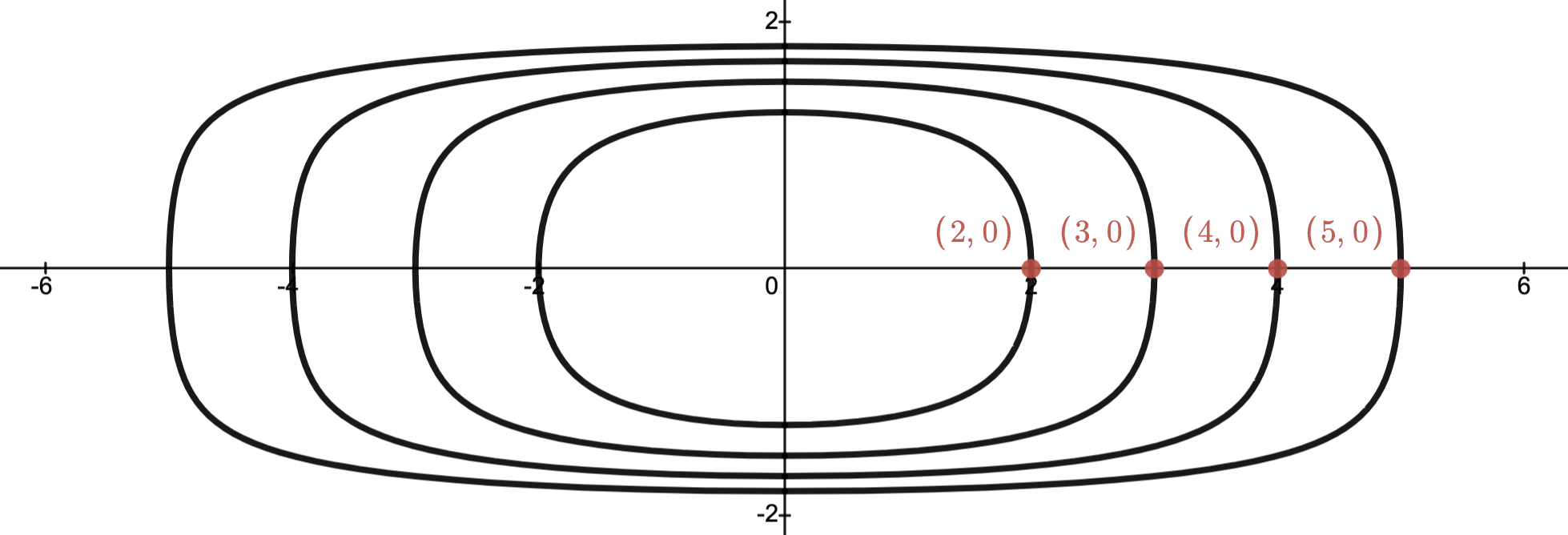
-Sublevel set:
the set

 with
with  .
.Each shade of gray indicates a new sublevel set and of course
 for
for  .
.

-Superlevel set:
the set

with .Each shade of gray indicates a new superlevel set and of course
 for .
for .
Proposition. If
is convex, then the sublevel set  is convex for all .
Equivalently, if
is concave, then the superlevel set  is convex for all
  .
.
Proof.
Want to show: implies
  for all .
If
, then  and so convexity of gives

and hence
as desired.
Graphs
Fix a function.
Graph:
the set

 is given below.

Epigraph:
the set 
is given below.
Hypograph:
the set

is given below.
Proposition.
is convex iff  is convex.
Equivalently,
is concave iff  is convex.
Proof. (sketch)
We consider the case for simplicity.Step 1. ()
Suppose is convex and let  be distinct points.
If
both lie on a vertical line, then clearly  for ; thus, suppose otherwise.
Let
 be the line passing through and let
  be the two intersection points of with the graph of .
(If at most one intersection point exists, then it is easy to see that the line connecting
and  is in
is in  .)
.)By convexity of
, the line formed by  for lies in , which is enough to conclude the line given by
  for lies in
  .
.This shows
 is convex.
Step 2. ()
Suppose now is convex.Let
be two distinct points on the graph of .Then
 .
.But convexity of
implies the line formed by  for lies entirely in .
This is enough to conclude
is convex.
Convex Calculus
The following list details some operations and actions that preserves convexity.The main point: to conclude a function
is convex, often one verifies may be built by other convex functions using, for example, the operations below.N.B.: Conclusions only holds on common domains of the functions.
Conical combinations:


Weighted averages:


Affine change of variables:


Maximum:

Supremum:


Justification.
For, there holds

Example.
Let

, the mapping  is affine and hence convex.
Thus

Infimum:


Fenchel conjugation
Let be given (not necessarily convex).
Fenchel conjugate:
 .
.N.B.:

 for which
  is bounded above on as a function of .
Intuition.
Suppose is a differentiable convex function denoting the cost to produce items.
For a given unit price
 , the profit of selling units is

 is just the optimal profit for selling at price
  .
.N.B.:
convex implies  is concave for each .
Thus,
 is maximal at satisfying
  , i.e., when
  .
.Viz.: the
where has slope  .
.The tangent line through
 is then given by
  .
.Lastly, note that the
-intercept of this line is  ,
,
Remarks
-
Often
is just called the conjugate function of
-
Since
is the supremum of a family of affine functions,
(Follows from Convex Function Theory.Convex Calculus. - If
-
-
,
.
-
Example.
We will compute the conjugate function of

Thus, let

Case  :
:
 is unbounded on
  since
since


Case  :
:
Compute

 maximizes
  and so

Case  :
:
Compute

 and so

Conclusion:
Since

only for  , it follows that


 .
.
Legendre Transform
Let be convex, differentiable and with  .
.Then, the Fenchel conjugate
of is often called the Legendre transform of .Proposition. If
as above, and  , then

Proof.
Step 1.
Let


is a sum of concave functions and hence concave.
Step 2.
Using Step 1. and


maximizes  .)
.)
Step 3.
Letting satisfy


Example 1.
Let

 , let
, let


in a previous example.
Example 2.
Fix and let


Step 0.
Observe-
(Justification)
Consider case.
Let.
Thus.
Easy now to see.
implies
is invertible since then
.

Step 1.
Using


Step 2.
Let .
.By preceding proposition and Step 1., there holds

Other Notions of Convexity
There are two other important notions of convexity that we will return to if needed.Let
be given.Quasiconvexity:
and the sublevel sets

 .
.Features:
- Quasiconvex problems may sometimes be suitably approximated by convex problems.
- Local minima need not be global minima
Log-convexity:
 on and
  is convex; equivalently

Generalized Convexity
Let be a proper cone and let
  .
-convexity: for all
.
-convexity: for all  and , there holds

-convexity: for all  and
and  , there holds

Examples
-
(CO Example 3.47)
Let.
Then-convex iff:
and
, there holds
which holds iff
for each, i.e., iff
-
(CO Example 3.48)
A functionis
-convex iff :
N.B.:.
-
this is a matrix inequality and
-convexity is often called matrix convexity.
-
is convex for all
.
-
The two functions
are matrix convex.
-
this is a matrix inequality and


Basics of Optimization Problems
General Optimization Problems
By an optimization problem (OP) we mean the following:


Feasibility
Consider an (OP) as above.Feasible point: those
 satisfying

 consisting of the feasible points.
Feasible problem: A problem with nonempty feasible set, i.e.,
 .
.
Infeasible problem: A problem with empty feasible set; i.e., there are no
 which satisfy the inequality and equality constraints.
Remark.
-
A feasible problem need not have a solution; e.g.,
- An infeasible problem never has a solution–there are no parameters
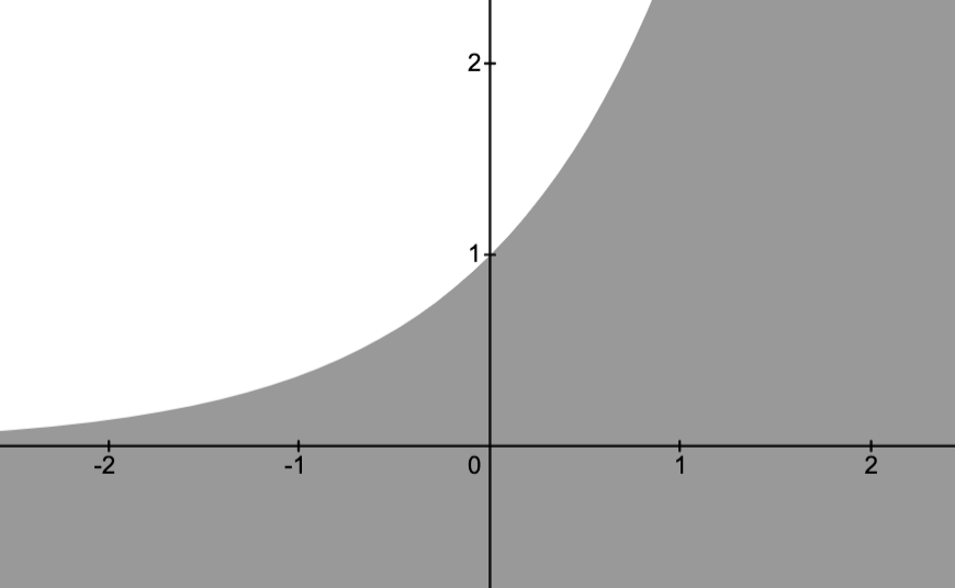
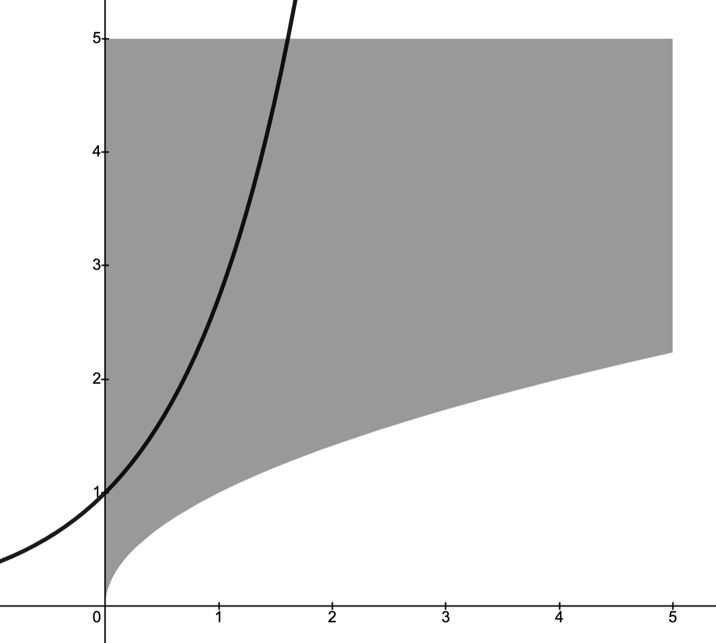
Basic Example
Consider the problem

The objective function is

The inequality constraint functions are

The domain of the problem is

The feasible set:
Let

Note that the darkest region given by
 is the feasible set.

Can we solve the problem?
Noting-
as
approaches a point on the circle
, and
- such sequences exist in the feasible set,
The Feasibility Problem
Feasibility problem: Given an (OP) with


Example 1.
The problem

This is depicted below.
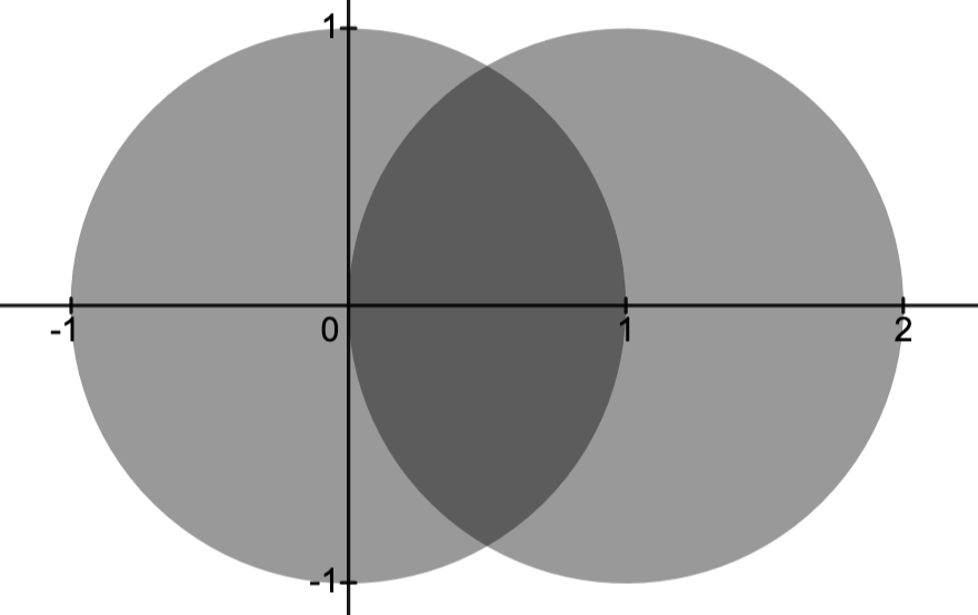
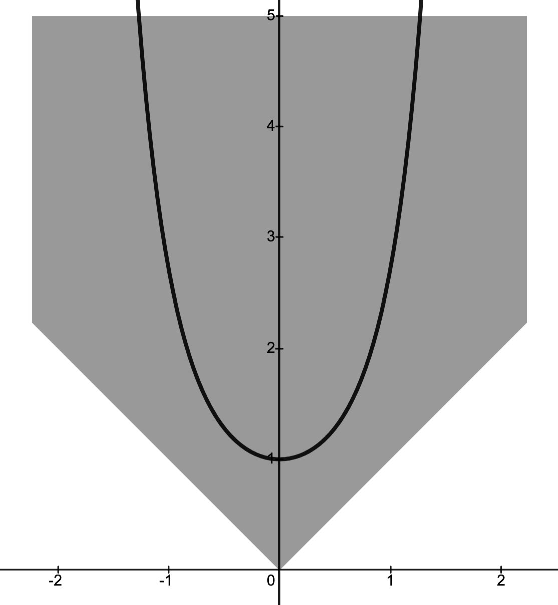
Example 2.
The problem

 lies outside of the intersection of the two disks.
This is depicted below, where the red circle is given by
.

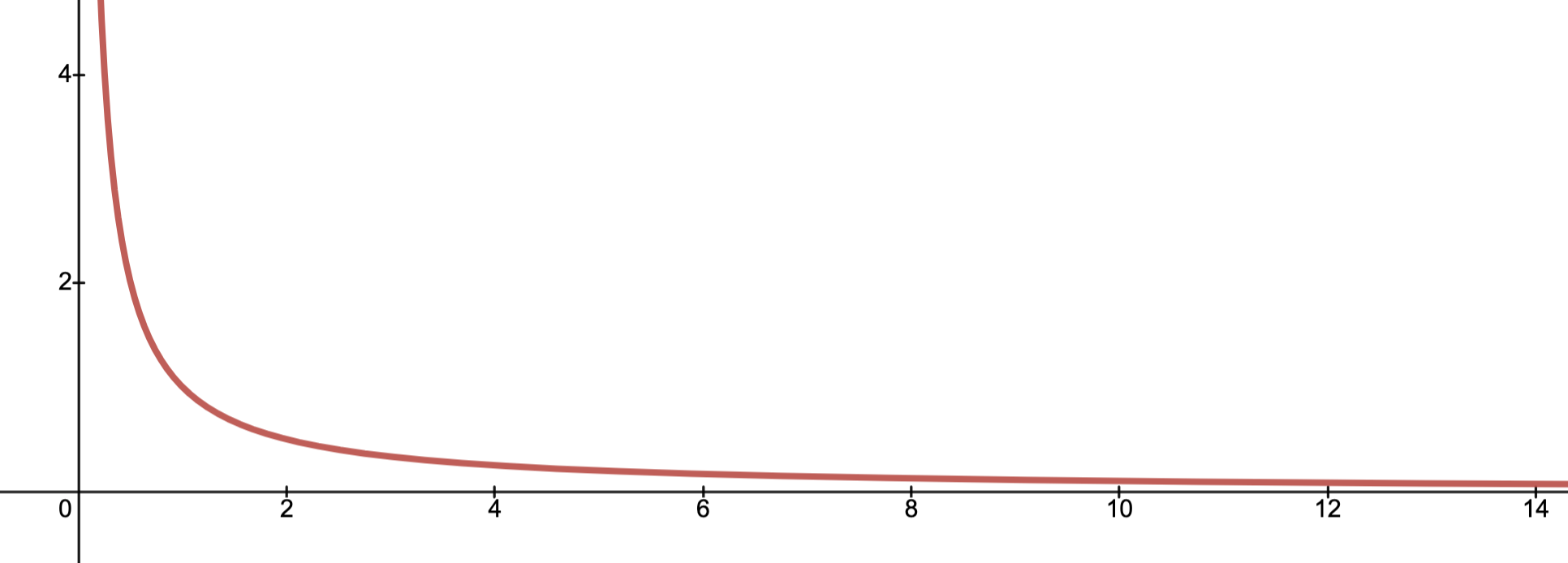
Optimal Value and Solvability
Recall:

Optimal value:
The value

 is the largest
  such that
  for all
  .
.N.B.:
 .
.
Example:
Below depicts the graph of on
on  .
.Evidently,
 .
.
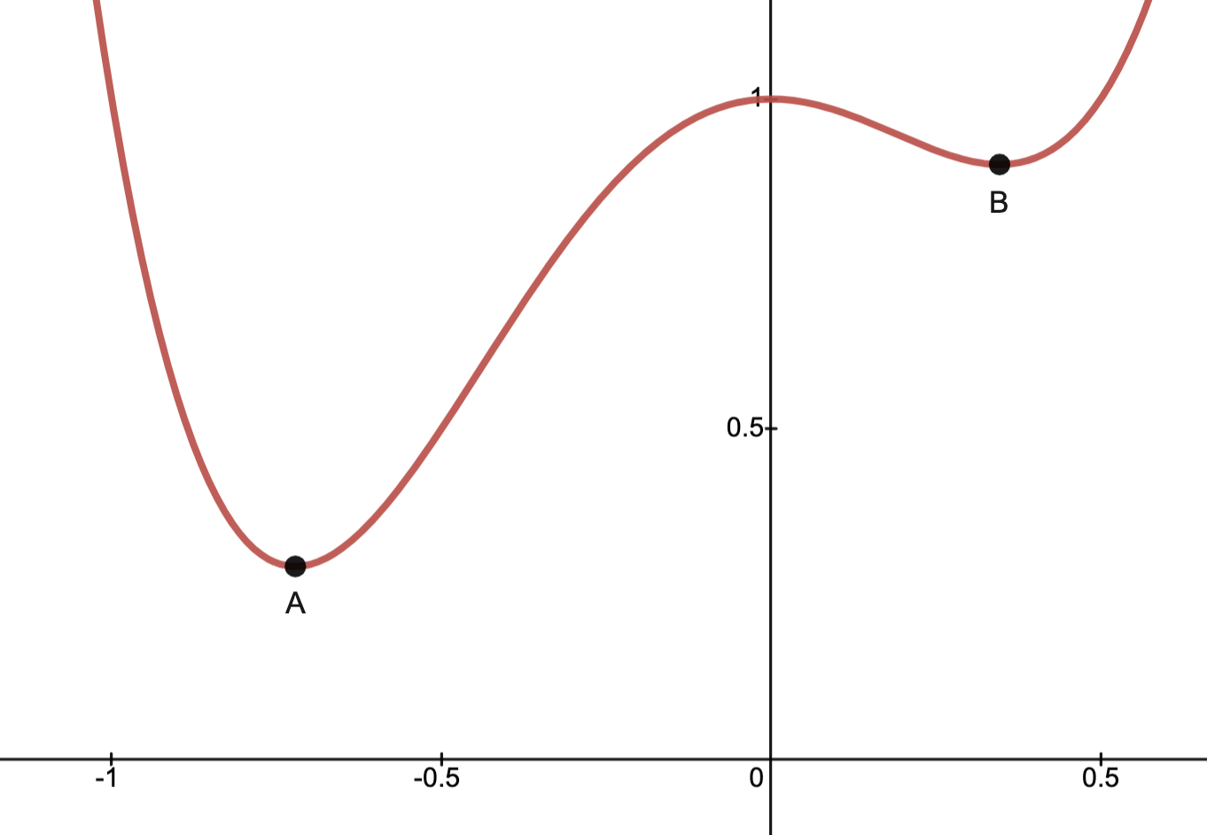
Solvable:
When the problem satisfies
there exists 

 is attainable.
Example:
Below depicts the graph of a quartic .
.The problem of minimizing
on is solvable with solution given by the minimal point .N.B.: Point
is a local minimum and hence does not give a solution.
Remarks.
-
iff the (OP) is solvable.
Indeed,is not well-defined unless the (OP) is solvable.
-
if
if the OP is infeasible.
Standard Form
Optimization problems need not be placed in the form we defined them.We therefore introduce the following definition.
(OP) in Standard form:

Example: Rewriting in standard form.
We can recast more general optimization problems in standard form; e.g., consider

(noting
)
for
for
Equivalent Problems
Suppose we are given two OP’s: (OP1) and (OP2).We say (OP1) and (OP2) are equivalent if: solving (OP1) allows one to solve (OP2), and vice versa.
N.B.: Two problems being equivalent does not mean the problems are the same nor that they have the same solutions.
Example.
Consider the two problems:
![\begin{cases} \text{minimize} & f(x) = x^2\\ \text{subject to}& x \in [1,2] \end{cases} \quad \text{and} \quad \begin{cases} \text{minimize}&g(x) = (x+1)^2+1 \\ \text{subject to}&x \in [0,1] \end{cases}.](https://s0.wp.com/latex.php?latex=%5Cbegin%7Bcases%7D+%5Ctext%7Bminimize%7D+%26+f%28x%29+%3D+x%5E2%5C%5C+%5Ctext%7Bsubject+to%7D%26+x+%5Cin+%5B1%2C2%5D+%5Cend%7Bcases%7D++%5Cquad+%5Ctext%7Band%7D+%5Cquad++%5Cbegin%7Bcases%7D+%5Ctext%7Bminimize%7D%26g%28x%29+%3D+%28x%2B1%29%5E2%2B1+%5C%5C+%5Ctext%7Bsubject+to%7D%26x+%5Cin+%5B0%2C1%5D+%5Cend%7Bcases%7D.+&bg=ffffff&fg=111111&s=3&c=20201002)
![x^\star \in [1,2]](https://s0.wp.com/latex.php?latex=x%5E%5Cstar+%5Cin+%5B1%2C2%5D+&bg=ffffff&fg=111111&s=3&c=20201002)

![[1,2]](https://s0.wp.com/latex.php?latex=%5B1%2C2%5D+&bg=ffffff&fg=111111&s=3&c=20201002)
![x^\star - 1 \in [0,1]](https://s0.wp.com/latex.php?latex=x%5E%5Cstar+-+1+%5Cin+%5B0%2C1%5D+&bg=ffffff&fg=111111&s=3&c=20201002)

![[0,1]](https://s0.wp.com/latex.php?latex=%5B0%2C1%5D+&bg=ffffff&fg=111111&s=3&c=20201002)
Indeed, if we find the solution
 to the first problem, we readily obtain the solution
  to the second problem, and vice versa.
Change of Variables
Suppose is an injective function with
  .
.Then, under the change of variable
 , we have


.Moreover, injectivity may be dropped.
Justification.
Indeed,-
if
solves (OP2).
(More generally,such that
solves (OP2).)
-
if
solves (OP1).
Example
Consider the problem

 .
.


Eliminating Linear Constraints
Let, and a solution to .Let
 be such that
  .
.Then
iff  for some
  .
.
Consequently


 many variables.
(Recall:
many variables.
(Recall:  .)
.)
Justification.
Indeed,- if
with
solves (OP2), and
- if
solves (OP1)
Example.
Consider the minimization problem

by simply using  .
.But, to match with above: let


 , and so

Therefore, the minimization problem becomes

 with optimal value
  .
.
Thus, the original problem has solution

Slack Variables
Given with  , then there is a variable
  such that
  ; such a variable
  is called a slack variable.
Using slack variables
 , the problem


Remarks.
-
All of the
-
Let
be the feasible set of (OP1) and
that of (OP2).
Thenand
; i.e., the feasible sets are not the same object.
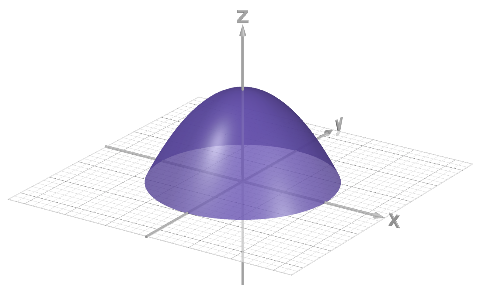
- Example: in the images below, the disk depicts a feasible set
and the paraboloid-type set depicts the feasible set
with slack variable
.
N.B.: the permissible

Main point:
Solving the system of equations

 may be easier than solving the system of inequalities

Example.
Consider

 satisfying


 is just a matter of solving a system of equations and choosing those
  with .
Moreover, one can solve the problem

to obtain solutions to (OP2), and hence (OP1).
Epigraph Form
Recall: .
.The optimization problem

 subject to constraints is equivalent to finding the smallest such that
  for some feasible .
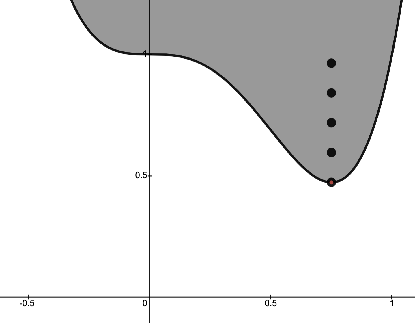
Proof by picture.
The dark curve and shaded region below indicate the epigraph of a function.The red dot indicates the minimum point
 .
.The black dots indicate points
 for different values of .
Evidently, the smallest
 for which
  is given by
  .
.
Fragmenting a Problem
Proposition. Given and sets
  with
with  let
let


 for any real number
  .)
.)
Viz., to minimize a function on a set
 , one may instead minimize over pieces of
  and then take the minimum optimal value of this procedure.
Example.
Consider the (OP)

 and where the feasible set is depicted below.
 into three regions
  as indicated below.

 , and let
  be the optimal value for (OPi).
Using the preceding proposition, the optimal value of (OP) is given by

Basics of Convex Optimization
Convex Optimization Problems
Abstract convex optimization problem: A problem involving minimizing a convex objective function on a convex set.Convex optimization problem: a problem of the form

-
-
and
are fixed.
Some Remarks
Remark 1.
As defined, a (COP) is an (OP) in standard form; naturally, there are nonstandard form (OP)’s equivalent to (COP)’s.E.g., the abstract (COP)


Remark 2.
We emphasize: the equality constraints are assumed to be affine constraints.Moreover, the equality constraints


Remark 3.
The affine assumption on the equality constraints can be lifted at the possible expense of an intractable theory/numerical analysis.E.g., if
 is quasilinear, then
  defines a convex set.
Remark 4.
Generally, convex does not imply the level set is convex; e.g.,
  gives a sphere.
Remark 5.
The common domain

Optimality for Convex Optimization Problems
Assume throughout that is the objective function for some given (COP) and that is the feasible set.
Proposition 1. If
is a feasible local minimizer for a (COP), then it is the global minimizer for the (COP).
Proof.
We will follow a proof by contradiction; i.e., we will show that assuming is not a global minimizer leads to a contradiction.
Step 1.
being a feasible local minimizer means  and that there is a
  such that

 for all
  with a distance at most
  of .
of .
Step 2.
Supposing is not a global minimizer, then there exists  such that
  .
.By choice of
, there must also hold  .
.
Step 3.
Set

by Step 2. and so since is convex.It follows that

Step 4.
Since is a convex combination of feasible points, since is convex and since  , there holds

minimizes on


must be a global minimizer.
is differentiable on , then is a minimizer iff for all there holds

Proof.
Step 0.
N.B.: since is differentiable and convex on , then for each  there holds

Step 1.()
Suppose is a minimizer and suppose for contradiction that

.Set
 , noting that
  since is convex.
Using

is decreasing near  in the direction
  and so
  for small .
Since
, this contradicts being a minimizer.
Additional justification
Since defines a line passing through with direction
  , it follows that
  is the directional derivative in direction
  , i.e.,
  .
.
Step 2.()
Supposing

and using the first order characterization at , namely,


; i.e., that is a minimizer for the problem.
is differentiable and  (equivalently, there are no nontrivial constraints),
  is a minimizer iff

Proof.
By Proposition 2., we have that is a minimizer iff

 .
.
Differentiability of
requires  is open and so, for small , there holds


 iff .
iff .
Some Examples
Example 1.
Let


 implies is convex.
C.f.,Convex Function Theory.Second Order Characterization. By the preceding corollary, we have
is a solution to (OP) iff

 .
.Three cases:
is the unique solution to (OP);
and
has an affine set of solutions.


Example 2.
Let


satisfying  is a minimizer iff

satisfying  .
.Two cases
is an inconsistent system
,
for some
.


In case 2., we have

 is a linear space, this is only possible iff


 and so this condition means there exists
  such that

Linear Programming
Linear program: a (COP) of the form


is a polyhedron (see below).
Recall ( ):
):
For  the vector inequality


Different than:
 satisfying the matrix inequality
  , which means
  is positive semidefinite.
Determining the Feasible set:
Step 1. ()
Given  ,
,  , then

or empty.
Step 2.
Given , then

.
Step 3. ( )
)
Given


Step 4.
Steps 1. and 3. imply the feasible to (LP) is the finite intersection of half spaces and an affine space, i.e., is a polyhedron.(c.f. Convex Geometry.Polyhedra.)
Example.
Let


and the graph of the objective function over are indicated in the image below.
Remarks.
-
Given
, have equivalent problem with objective
.
Indeed,
WLOG: can assumeto solve problem.
-
Since
one also calls the problem of maximizingover a polyhedron a (LP).


Example: Integer Linear Programming Relaxation.
Integer Linear Program: an (OP) of the form


 is suitable for parameters which take on discrete quantities.
N.B.: An (ILP) is not a convex problem, but may be approximated by one (see below).
The feasible set
Let

Then
is just the collection of integer vectors in the polyhedron

Example. Consider an (ILP) with constraints given by
 satisfying

(the collection of dots) and polyhedron (shaded region).
Remarks.
-
Can of course also impose equality constraints
-
If we impose
, then the problem is called a boolean linear program:
Suitable for when coordinates of
Can also useinstead.


Relaxation of (ILP)
The LP

Important points:
-
The “tightest” convex relaxation is given by
Generally speaking, finding the convex hull is not an efficient way of approaching (ILPs). - The relaxation (LP) of (ILP) is generally easier to solve, though exact algorithms exist for (ILP).
-
If
then.
(Indeed the relaxation has larger feasible set.) -
If
solves the (LP), then it solves the (ILP).


Relaxation of (BLP)
Explicitly, a (BLP) is of the form


N.B.: the relaxation
![F \to \{x \in [0,1]^n: Gx \preceq h \}](https://s0.wp.com/latex.php?latex=F+%5Cto+%5C%7Bx+%5Cin+%5B0%2C1%5D%5En%3A+Gx+%5Cpreceq+h+%5C%7D+&bg=ffffff&fg=111111&s=3&c=20201002)

Example.
Problem Given workers and
  locations with
  ,
,
- assign each worker to work at some location
- assign at most one worker to a location
- minimize cost of operation and transportation


Construct objective function
We find

 .
.Construct constraints
The constraint that
 are binary is of course natural for the problem.
Since each worker is selected only once, we have

 since the
  th location not operating means it cannot host a worker; thus we have
  .
.Formulate Problem
Putting everything together, the (BLP) formulation of the problem is

![\begin{cases} \text{minimize} & c^Tx + \text{tr}\,(C^TX)\\ \text{subject to} & x \in [0,1]^n\\ &X \in [0,1]^{m \times n}\\ &\sum_{j=1}^n x_{ij} =1, i = 1,\ldots,m\\ & x_{ij} \leq x_j, i=1,\ldots,m,j=1,\ldots,n \end{cases}.](https://s0.wp.com/latex.php?latex=%5Cbegin%7Bcases%7D+%5Ctext%7Bminimize%7D+%26+c%5ETx+%2B+%5Ctext%7Btr%7D%5C%2C%28C%5ETX%29%5C%5C+%5Ctext%7Bsubject+to%7D+%26+x+%5Cin+%5B0%2C1%5D%5En%5C%5C+%26X+%5Cin+%5B0%2C1%5D%5E%7Bm+%5Ctimes+n%7D%5C%5C+%26%5Csum_%7Bj%3D1%7D%5En+x_%7Bij%7D+%3D1%2C+i+%3D+1%2C%5Cldots%2Cm%5C%5C+%26+x_%7Bij%7D+%5Cleq+x_j%2C+i%3D1%2C%5Cldots%2Cm%2Cj%3D1%2C%5Cldots%2Cn+%5Cend%7Bcases%7D.+&bg=ffffff&fg=111111&s=3&c=20201002)
Quadratic Programming
Quadratic program: an (OP) of the form


 , then the problem is convex (see remarks).
Remarks.
-
As for (LP), the constraints
describe a polyhedron.
-
Given
WLOG: can assume
-
If
then,
Thusimplies
N.B.: The factoris just a convenient normalization.
-
The generalization
results in quadratically constrained quadratic programming (QCQP).
Imposingensures the (QCQP) is convex.
(C.f., Convex Function Theory.Level Sets.)
-
The generalization
also results in a (QCQP), but this can break convexity.
E.g., The quadratic constraints
result in a (BLP) since these constraints enforce, respectively.
-
There holds
-
The assumption
(i.e.,
) is not a serious restriction.
Indeed, first note that, sinceis a scalar, we have
.
Let.
Thus,
where.
Lastly, observe the symmetry of:
.
Thus every quadratic
has a “symmetric representation” of the formwith
.


Example: Least Squares
Least squares: an unconstrained (QP) of the form

 and
and  .
.Features:
-
WLOG: may assume columns of
.
-
N.B.: a least norm solution to (LS) is generally given by
where,
is the pseudo-inverse (aka Moore-Penrose inverse) of
-
Under the WLOG assumption, there holds
.
Recall (definition of  )
)
For , the notation  means the vector norm

 .
.
Rough Justification of WLOG
Let


Therefore, we may write

Computing


Therefore, a (LS) problem with matrix of size
 is equivalent to a (LS) problem with matrix of size
  .
.This argument holds in general: if
has linearly dependent columns, can use change of variables to ensure linear independence.
Remarks.
-
If
-
If
, where “best” is chosen to mean in terms of the vector norm
-
While minimizing
is equivalent to minimizing
ensures
(C.f.:is not differentiable at
, but
is.)
Solving the (LS)
Step 1. (The problem is convex)
The objective function


 , observe:
-
and so
, i.e.,
is symmetric;
-
for all
i.e.,,
.
Step 2. (The critical points)
We compute

 iff
iff

Step 3. (The solution)
By corollary proved above: is a solution iff .Moreover,
having linearly independent columns ensures that is invertible:
- linear independent columns
iff
.
- Since


Lastly: since

 is invertible, we conclude that the solution to the (LS) is
Example: Distance Between Convex Sets
Let be convex subsets.
Nearest Point Problem (NPP): Among
 , which pair minimizes the distance
  ?
?
The (NPP) may be expressed as a standard form (COP).
Indeed, supposing

 convex, then the (NPP) for
  is the (COP)


 iff .
iff .
When the
are polyhedra, then the (NPP) is a (QP).Indeed, supposing

is the (QP) given by


Polyhedral Approximation.
Let be nonempty convex domains, not necessarily polyhedral.
Let  be polyhedral domains such that

![[P_1,P_2]](https://s0.wp.com/latex.php?latex=%5BP_1%2CP_2%5D+&bg=ffffff&fg=111111&s=3&c=20201002) and
and ![[Q_1,Q_2]](https://s0.wp.com/latex.php?latex=%5BQ_1%2CQ_2%5D+&bg=ffffff&fg=111111&s=3&c=20201002) provide (QP) relaxations of the (NPP) for
provide (QP) relaxations of the (NPP) for ![[K_1,K_2]](https://s0.wp.com/latex.php?latex=%5BK_1%2CK_2%5D+&bg=ffffff&fg=111111&s=3&c=20201002) and, respectively, provide upper and lower bounds for the optimal values for the original (NPP).
and, respectively, provide upper and lower bounds for the optimal values for the original (NPP).
Geometric Programming
Monomial function: given


Remarks.
-
Let
Since any monomial is a posynomial, we have.
-
If
then
Thusis a group and
a “conic representation” of
-
As usual, we use the language “writing in standard form” to refer to writing an equivalent (OP) written in the form (GP) above.
General (OPs) clearly equivalent to a (GP) may be called a geometric program in nonstandard form.
For example, the geometric program
with
is readily rewritten as a standard form (GP):


Rewriting (GP) as a (COP)
General (GPs) are not convex (e.g., ).
).However, any (GP) is easily recast as a (COP) via change of variable.
Step 1. (The change of variable)
We will write to mean the change of variable given by

Step 2. (Monomials  convex function)
Let

 :
:


 is convex since affine functions are convex.
Step 3. (Posynomial convex function)
For  , let
, let


Step 4. ((GP) (COP))
We explicitly write the (GP) as:


, this (GP) becomes the (COP)

Step 5. ((GP) in convex form)
At last, since exponentiation may result in unreasonably large numbers, it is customary to take logarithms, resulting in the geometric problem in convex form:

-
Concavity of
is too weak to break the convexity of
-
The constraints are equivalent since
Example.
(Taken from Boyd-Kim-Vandenberghe-Hassibi: A tutorial on geometric programming)Problem Maximize the volume of a box with
- a limit on total wall area;
- a limit on total floor area; and
-
upper and lower bounds on the aspect ratios
and
.

The volume of the box is


Construct contraints


Putting everything together, we realize the problem may be formulated as the following (GP):


is equivalent to minimizing  .
Therefore, the problem in standard form is given by
.
Therefore, the problem in standard form is given by

Semidefinite Programming
(Heavily influenced by Vandenberghe-Boyd Semidefinite Programming.)Linear matrix inequality (LMI): given


 , we write
  to mean is positive semidefinite, i.e.,
  for all
  .
.
Semidefinite program (SDP): an (OP) of the form


defines a feasible set which is convex and hence (SDPs) are convex problems.
Convexity of Feasible Set.
To see that (SDP) is a convex problem, first note: if


feasible and , the function


 , we conclude

feasible feasible for , i.e., the feasible set is convex.
Example 1. LPs are SDPs
Consider the (LP)


Given
 , define

Since
satisfies iff has nonnegative eigenvalues, we have

 are the components of .)
Therefore,
are the components of .)
Therefore,

Letting


Therefore, using


Therefore, defining


In conclusion, we have that the (LP)

Example 2. Nonlinear OP as a SDP
Consider the nonlinear (COP)


N.B.:
-
choice of domain (a halfspace) of objective and ensures convexity.
-
concave problem.

.
Goal: find a symmetric matrix-valued function


 , then

 , we have


Indeed, evidently,
 iff
iff


To make it clearer, introduce the notation

 matrices


Lagrangian Duality
Throughout, let (OP) denote a given optimization problem of the form

Recall:

The Lagrange Dual
Lagrangian: the function


, the function

Lagrange multipliers: the variables
 and
and  .
.The vectors

Lagrange dual function: the function


 satisfying

N.B.: as an infimum of affine functions,
is automatically concave.
Proposition. For


is the optimal value for the given (OP).
Proof.
-
Let
Then
-
Let
and
be arbitrary.
Then feasibility of
Consequently,
-
Therefore, for all feasible
and for arbitrary
and so
(Indeed,.
is a lower bound of


Lagrangian as underestimator.
(See CO 5.1.4)
Define the indicator functions


N.B.: if
is feasible and  , then


 is an underestimater of the objective function


In particular, for each
 , the problem

and provides an underestimation of the original (OP).Example 1
Consider the least squares problem


Therefore, the Lagrangian
for (LS) is


N.B.:

 is convex.
Consequently,


In conclusion,


 .
.
Example 2
Consider the linear program


-
equality constraints given by
.
-
iff
iff.

Therefore, the Lagrangian for (LP) is

Want to compute


.Therefore,
 satisfy

Therefore, the Lagrange dual is

In particular, for dual feasible
 , there holds

.
Return of Conjugate Function
Recall: given, its conjugate function is the convex function

Consider the the (OP)


The Lagrangian is

We may now compute the Lagrange dual in terms of the conjugate
 :
:


Appendix
Differentiating 
Given


 , we find


Differentiating 
Given


 , we find


Example.
Let


Differentiating 
Given , , define the scalar function 
Using the Taylor expansion

, we get


